An Explanation and an ANOVA Calculation Example
Our white paper regarding t-test calculations has been very popular. Those that use the t-test tool regularly have commented “I finally understand what it is all about.”
The natural question they ask me next is “have you done anything with the F-test?” It is another common tool and one that is equally misunderstood.
Due to popular request, here is our attempt at explaining the F-test tool, in the two possible methods of use.
Background on the F-test
As we are a company built around Design of Experiments (DOE), it is interesting that the F-test was developed by Sir Ronald Fischer – the god father of DOE! The “F” in F-test is a credit to him. Further, in the name of trivia, the modern day guru of DOE is George Box. He married Fischer’s daughter. A small world as they say! Before I started teaching DOE, I had a long conversation with George Box – gaining insights to better apply the DOE methods.
Now let us move on to the nuts and bolts of the test.
The F-test calculations are typically summarized in something called an ANOVA or ANalysis Of VAriance table. As the name implies, the calculations are performed using variance values or sub calculations. The typical format of the ANOVA table is shown below for a typical Design of Experiment application, but it is similar for other F-test applications.
| Source | Sum of Squares (SS) | Degrees of Freedom (DF) | Mean Square (MS) | F–Value (ratio> |
|---|---|---|---|---|
| Model | ||||
| Center Point | ||||
| Residual (error) | ||||
| Block | ||||
| Total |
The “source” terms are as follows – Model is the equation of study, Center Point is the middle of the design space, Residual is for the “left over” items from the model (or items not included in the model), Block is from the noise reducing variable (if used), and Total is just a grand sum of each column. This is possible as variances (squared values) have an additive property. This is a lot of terminology and it changes based on the usage. You just have to know the source that is relevant for you.
The column titles are defined as follows – Sum of Squares is the addition of squared values (the formula for these values depends on the question being asked), the Degrees of Freedom is a count of the pieces of information used to create the row item, and finally the Mean Square is the Sum of Squares divided by the degrees of freedom. An extension to the table is the F-Value (or ratio) which is simply the ratio of the calculation of interest divided by the residual (or estimate of random error). The “calculation of interest” could be comparing the model, comparing means or comparing center points to noise.
The F-Value along with the Degrees of Freedom for each item then allows calculation of a p-value, or percentage value. Like the t-test, a value of less than 5% is considered significant, or an indication that a difference exists. This value is often shown near the ANOVA table, but normally not in it.
Why use the F-test?
Essentially, the F-test compares two variances (which is the standard deviation squared) to see if they are equal. The calculation concept is similar to the t-test. While the ANOVA math is based on variances, depending how the calculations are performed, an F-test can either compare variances or compare means.
The F-test can address several questions:
- Is the model or equation meaningful compared to random noise (a variance comparison)
- Are the center points different than the linear prediction (a version of mean comparison)
- Are the means different at various levels (accomplishing the same thing as a t-test)
We will investigate both of the calculation approaches, comparing variances and comparing means.
F-test calculation method for Variance
Comparison As stated earlier, the format for showing all sums of squares and related statistical items for an F-test is called an ANOVA table. Again, this is a calculation example for a DOE case – and a short cut calculation method. The model chosen has 3 terms, which we will not specify for the purposes of our discussion:
| SS | DF | MS = SS / DF | |
|---|---|---|---|
| Model | 1262.5 | 3 | 420.8 |
| Residual | 54.5 | 3 | 18.17 |
| Block | 0.5 | 1 |
Where do these numbers come from?
We will start with the Sum of Squares (SS). It is calculated as: SS(effect) = N * effect2 / 4. To calculate the effect value, it is simply effect = A+(avg) – A-(avg), where A+(avg) is the average value for variable A at the high setting and A-(avg) is the average value for variable A at the low setting. N is the number of pieces of raw data, which for this DOE was 8.
The 3 original effects for the example model are 23, 10, and 1.5. They are the inputs to the table below and yield a total SS value of 1262.5.
| Effect | Effect Squared | SS calc |
|---|---|---|
| 23 | 529 | 1058 |
| 10 | 100 | 200 |
| 1.5 | 2.25 | 4.5 |
| SS = | 1262.5 |
Similarly for the residual, we have the following calculations:
| Effect | Effect Squared | SS calc |
|---|---|---|
| -5 | 25 | 50 |
| 1.5 | 2.25 | 4.5 |
| 0 | 0 | 0 |
| SS = | 54.5 |
Finally for the block, we have the following calculation:
| Effect | Effect Squared | SS calc |
|---|---|---|
| 0.5 | 0.25 | 0.5 |
| SS = | 0.5 |
The block is not required for the calculation we are performing, but is included for completeness of the ANOVA table.
The DF in the ANOVA table stands for Degrees of Freedom. It is a count of the pieces of information used for the calculation. For a DOE, the total amount of information available is one less than the number of test points. This is because when we are creating an equation (or model), our starting point is to calculate an average value. This reduces the available pieces of information by one. Thus, a simple 2 level, 3 factor full factorial DOE has 8 test data points. This leaves 7 pieces of information for the calculations and the other terms in the equation.
In our case, the block takes away another piece of information, leaving us with 6. The Mean Square (MS) equation is shown as the SS divided by the Degrees of Freedom. As we stated earlier, the model, or DOE equation, has 3 components. This means that 3 pieces of information are not used and are thus used to calculate the residual error.
Taking the values provided above, we can calculate the Mean Squared values column in the table. The F-test statistic is then the ratio of the MS values.
For this example model, we have the following:
F = MS(model) / MS(residual) = 420.8 / 18.17 = 23.16
Because the statistical test is asking if the model or equation is the same as noise, the only other option is to be larger than noise (it is not practical to be smaller than noise). Thus, F is a one sided statistic. Using the appropriate DF and a standard F table, we find that the alpha level (or p-value) is:
α = 0.0167 (using linear interpolation from a published F table)
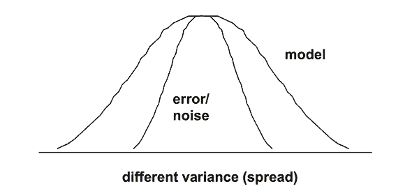
This means there is a low probability they are the same. Thus, we are to conclude (infer) the model is different than random noise. Since our objective is to build a model (create an equation), this statistical significance is good news! While there is more work to confirm a valid and useful equation, this is one of the initial hurdles. The graph below shows the concept of the F test.

From a DOE perspective, I will often say this means we have enough terms in our equation. However, we may have too many terms. Thus, we need to evaluate each term individually as the next step.
F-test calculation method for Mean Comparison
What about the factor effects calculation? That is DOE language for “mean comparison.” Why are we interested in this? While the previous calculation showed our equation was different than noise, we also need to ask the question “have we included too many terms in our equation?” An F-test for each coefficient in the equation (main effect and interaction terms) is required. Each term will add another row in the ANOVA table. The F-test calculation should match the t-test data shown in our other white paper. The Sum of Squares equation for this case is:
SS (factor) = Sum (n * (yk – z)2 )
where yk is the average for each factor level, z is the overall test average, and N is the number of samples at that test level.
Thus for our example we have the following raw data and summary statistics:
Low level for variable (factor) A (A-): 67, 61, 59, 52. This provides a 59.75 average (A-avg).
High level for variable (factor) A (A+): 79, 75, 90, 87. This provides a 82.75 average (A+avg).
Combining all 8 pieces of raw data, we have an overall average of 71.25.
For the main effect calculation for variable A, we have the following SS value:
4 * [(59.75 – 71.25)2 + (82.75 – 71.25)2] = 1058.
We are determining one piece of information (one coefficient), thus we have one DF.
Now, we need to determine our error component. The general equation is:
SS (error) = sum [y (each individual at the test level) – y (average at the test level)]2
However, in a DOE setting we can determine the noise component, an estimate of error, by summing the SS values from the effects not included in the model (equation). This begins to get deep quickly though really is straight forward.
In our example, we use the three smallest effects which are -5, 1.5 and 0. Each uses the same calculations as above. This yields a value of 54.5, with three (3) degrees of freedom. This leads to a MS value of 18.17.
Again, we calculate the F ratio from the Mean Squared values.
F = 1058 / 18.17 = 58.24
Using the appropriate degrees of freedom, we obtain a p-value of 0.0084 (again, using linear interpolation from a published F table). Because alpha is less than 0.05, we can assume these means are different for the main effect for A.
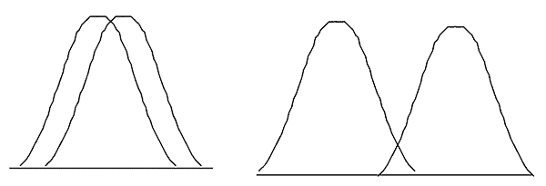
Similar to the t-test, we are comparing means. The picture below indicates the concept. If the data distributions overlap as seen on the left below, we would infer that the means are the same. If the data distributions have “minimal” statistical overlap as shown in the graph on the right below, then we would say that the means are different.

What is this doing for us? The value of F creates a confidence zone for the comparison of the means. Many people use a 5% value as a typical rule of thumb for α (alpha) which implies a 95% confidence for inferring the means are the same. Most people have performed this calculation, but hopefully it means a little bit more now.
We went through this long process to answer the question “is 82.75 different than 59.75”. Are we really surprised, looking at the raw data, that we say they are different? I don’t think so. In situations where it is not obvious, this numerical method will help us make an unbiased assessment of our data.
In our case, we would say that statistically there is a low probability that the means are equal. Thus the two means are considered to be different. We have to always determine if this difference is practically different, and for this data we can assume that they are practical differences for variable A. We would follow the same process for the other two terms in our equation, which are variable C main effect and the AC interaction.
Summary
In conclusion, you can now see where there are squared values created thus a variance calculation is taking place. How we use the data and how we group things will determine what we can infer. We can either compare variances or we can compare means. Each requires a different slice of the data – and many short cuts (or alternatives) exist to obtain comparable values.
Perry Parendo
Perry’s Solutions, LLC
651-230-3861
www.PerrysSolutions.com
 Ask a question or send along a comment.
Please login to view and use the contact form.
Great explanation…thanks for sharing
Thanks for the recognition, Arinze! My pleasure.
that is a fantastic explanation
Thanks, Isaac! Seems it can be a reasonably simple concept.
thanks for this simplified explanations. Iam still struggling to calculate relationship of three variable using the anova.
The example shows only 2 variables as you noticed, but the same principles work for additional variables. With computer software available, doing it by hand is not required for practical applications. I provide the description to help understand the background, but the key is always on data generation and decision making.