A t-test Example
The basis of DOE analysis is comparing two samples. This methodology can be used just as well for changing one variable or more than one variable as in DOEs. Comparison of means is as simple as the t-test.
Some people initially feel intimidated considering the connection of DOE with statistics. Once they understand it in simple terms, the topic comes together for them.
So let’s see if we can accomplish that for you now.
A t-test Description
First, what is the t-test about? It is used to compare two sample means within a confidence zone. Statistically speaking, it is a test of the Null Hypothesis. It is also known as “Student’s” t distribution. But we are keeping things simple, so think about it as comparing two means.
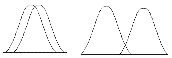
This can be shown graphically below. The figure on the left represents something that most people would call “the same”. Statistics will put numbers on it, but it should make sense by looking at a picture. The figure on the right shows “different”. Again, I think you’ll agree it is obvious in this case.

So why does it get complicated when we add numbers to it? I think it is only because we lose the fact there is a graph behind it. The numbers by themselves don’t mean much if you forget the source of the number. Of course, reality may have different standard deviations – but that can easily be accounted for mathematically. So let’s review the method of calculation.
The “t-score” is arrived at as follows:
t-score = (mean1 – mean2) / (standard deviation / n1/2)
Where n is the sample size.
What does this do for us? The value of t creates a confidence zone for the comparison of the means. Many people use a 5% value as a typical rule of thumb for α (alpha) which implies a 95% confidence for inferring the means are the same.
A DOE t-test Example
Most people have performed this calculation, but hopefully it means a little bit more now. Let’s take a look at some data. This is a DOE t-test, which is somewhat simplified.
We will use the following two data sets:
Low level for factor A (Alow): 67, 61, 59, 52
This provides a 59.75 average (Alowavg) and a 6.18 standard deviation s(Alow).
High level for factor A (Ahigh): 79, 75, 90, 87
This provides a 82.75 average (Ahighavg) and a 6.95 standard deviation s(Ahigh).
We need to account for the difference in standard deviation between the two populations. Statistically, this is called a “pooled standard deviation”. For us, let’s just say we are computing a weighted average of the variance (the standard deviation squared). Because we have the same number of samples for each level of factor A, this becomes a simple equation.
spooled2 = ( s(Alow)2 + s(Ahigh)2 ) / 2
Now, we just need to plug in the remaining data from the problem. Again, this is a simplified equation for a DOE situation.
t-score = (Ahighavg – Alowavg) / (spooled / (n/4)1/2)
= (82.75 – 59.75) / (6.58 / (8/4)1/2) = 4.94
In this case, we have 6 Degrees of Freedom (DOF) knowing that DOF = n – 2 for a DOE. Taking this t-score to a t-table (see the partial t-table below), we interpolate to find the probability value also called a p-value.
Partial t-table
| Probability (two tailed) | ||
|---|---|---|
| DOF | 0.005 | 0.001 |
| 6 | 4.317 | 5.959 |
This t-score provides roughly an α = 0.003. Because alpha is less than 0.05, we can assume these means are different. Now, let’s think about it again. We went through this long process to answer the question “is 82.75 different than 59.75”. Are we really surprised, looking at the raw data, that we say they are different? I don’t think so.
Statistically, we would say there is a low probability they are equal means. Thus the two means are considered to be different.
Summary
In conclusion, all we are trying to do with a t-test is compare two means – are they the same, or different. In DOE, we are hoping to find different means because those things will change (improve) our product or process performance if we set them to the proper level.
Current Contact Information
• PerryParendo
• 651-230-3861
• Perry@PerrysSolutions.com
• www.PerrysSolutions.com
 Ask a question or send along a comment.
Please login to view and use the contact form.
Leave a Reply