The operating characteristic curve, OC curve, visualizes a sampling plan.
At times, we select a sample from a group of items and evaluate them. Does this lot of widgets meet the specifications? Does this batch measure up?
Using lot sampling we can avoid 100% inspection, which may not be possible (destructive testing) or feasible (cost, time). Yet, not all lot sampling plans are the same. We can use OC curves to compare plans, design the right plan for our situation, and to explain the statistics behind a sampling plan.
Once we construct an OC curve we then have to be able to read the curve.
While not difficult there are few things to consider as you read the curve. Let’s explore two sampling plans and their OC curves to see what the curves tell us about the plans.
The Initial Lot Sampling Plan
Let’s say we will periodically receive a shipment of widgets. There are 1,000 said widgets per shipment. We know the supplier’s manufacturing process is not in control and they ship a lot with more than 5% defective items on occasion. Ideally, we want to have fewer than 1.5% defective widgets.
So, we set up a simple lot sampling plan. Draw 50 random widgets from the shipment of 1,000 and inspect them. If none fail to accept the lot, if one or more fail, reject the lot.
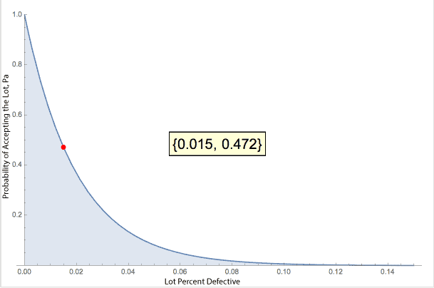
The OC Curve for this plan looks like this:
The red dot and bracket numbers indicate that if the actual, generally unknown, lot defect rate is 1.5% we would accept this lot a little less than half the time, 47.2%. The x-axis is the lot percent defective. It is unknown, hence the desire to sample the lot to determine the lot defect rate.
The curve provides the relationship given a lot defect rate of this sampling plan accepting the lot. In this case, even when the lot meets our target of 1.5% there is a reasonable chance that we would reject the lot, 1 – 0.472 or better than a 50% chance of rejection. Not all that good is it.
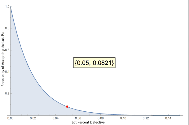
On the other hand, if the actual lot has a 5% defect rate this sampling plan would have less than a 10% chance of accepting the lot.
In short, the lot has to enjoy a low failure rate for this sampling plan to have a high chance of accepting the lot. And, if the lot has a high defect rate burden, this plan would most likely reject it.
When failures are OK
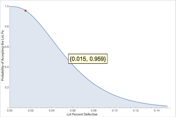
Now let’s look at a slightly different sampling plan for the same situation of inspecting a lot of 1,000 widgets. Let also select 50 random widgets from the lot and conduct our inspection. This time, if we have 2 or fewer failures we still accept the lot. Notice the OC Curve changes shape.
Now, if the actual, unknown lot defect rate is 1.5% we have a 95.9% chance of accepting the lot. This means we have less than 5% chance of rejecting a ‘good’ lot. This is much better than the 47.2% chance of lot acceptance with the previous plan.
Yet, what else happens? Take a look at what happens when the lot actually has a 5% defect rate.
Now we have a 54.4% chance of accepting the lot. The previous plan had less than a 10% chance. This plan favors the producer. Good lots are accepted and poor lots may still pass, too. The previous plan favored the consumer. Really good lots are accepted and poor lots are nearly always rejected.
Summary
The sample creates an estimate of the defect rate for the lot. The chance the sample accurately represents the lot defect rate is left to chance (random sample). Of course, sampling more widgets improves the accuracy, yet you should also consider the accept/reject rules, too.
Being able to read the OC curve helps you understand how well your sampling plan will both accept good lots and reject bad lots, and the chance of making an error based on the results of the sample testing. Plot the plan. See what it has to tell you.
Related:
OC Curve with Binomial Method (article)
OC Curve with Hypergeometric Method (article)
Sequential Sampling by Attributes (article)


 Ask a question or send along a comment.
Please login to view and use the contact form.
Thank you so much for your instruction.
It is really easy understand.
The instruction is really good to explain the curves. There is one point I didn’t undertand. How did the OC curve change? Lot size and sampling number are same but the curve shape is different.
I try to prove a case including 7680 lot size with 200 sampling. I didn’t find any fail item during inspection. According to OC curve I have a probability to accept the lot is %5,07 (n=200, C=0, real fail item = %1,48). That means I have a huge possibility to reject the lot but in reality I didn’t find any fail item. I have to explain this situation to the customer.
The second curve in your instruction may explain our situation but the curve I have is like the first one. Can you help me to clarify the problem? How can I change the curve shape?
near the bottom of the article are two links to articles that describe how to construct OC curves. One is OC Curve with Binomial Method and the others is OC Curve with Hypergeometric Method
hope that helps
cheers,
Fred
I never understood the meaning of OC curve until read this article. Thanks Fred!