Guest Post Prepared by Eugene Danneman, Wind Wear LLC
Introduction
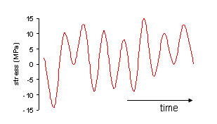
Analyzing and visualizing data that is related to equipment wear-out (fatigue stage) over a specific time span is a challenge. Analyzing systems, equipment and components exposed to spectrum loading as opposed to uniform cyclical loading that span years or decades or centuries requires a special approach. Think of roads, bridges and other assets with long life spans that are susceptible to wear out mechanisms caused by external and internal loads, varying load durations, temperature swings and corrosion.
For complex processes that consist of many pieces of equipment and components, it is often useful to take time history data and convert it to a count of the tensile and compressive cycles that equipment was exposed to. That data may be mechanical, thermal, electrical, chemical or some combination of forces that cause the irreversible degradation of the component material being studied. Historical throughput or production data is often the easiest to gather and analyze for “40,000 foot” cycling studies where one significant digit and one order of magnitude accuracy is adequate.
The rain-flow-counting algorithm (also known as the “rain-flow counting method”) is used in the analysis of fatigue data in order to reduce a spectrum of varying stresses into a set of simple stress reversals.1
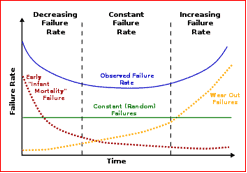
The fatigue phase of a product’s life cycle bath tube curve is characterized by an increasing failure rate.2
When we understand the physics of failure(s) caused by cycling forces, the wear out phase can often be postponed using effective predictive and preventative maintenance methods.
Delaying wear-out failures increases useful life; avoids or mitigates catastrophic events and reduces process production costs.
The American Society of Testing and Materials Standard ASTM E 1049-85 “Standard Practices for cycle counting in fatigue analysis” has many cycle-counting algorithms. One of them is the rainflow cycling counting algorithm created by Downing and Socie.
There are many software solutions using rainflow counting algorithms available for your use. I have been using the StoFlo freeware rainflow cycle counting Excel template.4
Example
The following example uses production data for a conventional thermal power plant with a design maximum output of 767 Megawatts/hour that was in continuous production for the study period of 365 days (8,760 hourly data points).
The raw data for this example starts with hourly production data (00:00:00 hour = 771.47 Megawatts) which is loaded into the StoFlo rainflow cycle counting Excel template. Table 1 show the format used.
Table 1 -Data format (Hour and Stress Value – Megawatts)
| 00:00:00 | 771.47 |
| 01:00:00 | 759.72 |
| 02:00:00 | 744.47 |
| 03:00:00 | 627.38 |
| 04:00:00 | 610.74 |
| 05:00:00 | 527.55 |
| 06:00:00 | 651.00 |
| 07:00:00 | 712.61 |
| 08:00:00 | 774.15 |
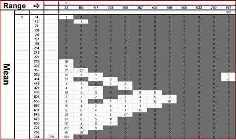
The output of the StoFlo cycle counting produces an analysis output (Table 2) showing the range of each hourly cycle and the average production load for each “rainflow” count.
Table 2 – Range and Mean rainflow cycle count for XYZ Power Plant
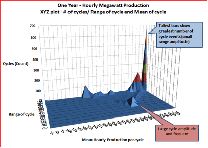
Table 2 is converted to a Excel software 3D graph with the cycle counts on the Y vertical axis, range of cycle on the Z axis and the average hourly production per cycle shown on the X axis.
Observations
- The tallest bar of the 3D plot is located in the right rear (over 650 cycles between a load of 756 and 784.
- An unusual pattern is shown at about 525 Megawatt with a production swing of ~500 Megawatts in one hour for about 50 cycles in this one year study period. Further study is needed to understand the magnitude of damage that could be occurring from changes in temperature, pressure, external forces and/or corrosion mechanisms at the component level.
This simple analysis approach provides the starting point to drill deeper where cycling related forces could be causing irreversible damage. It provides a graph that is easy to understand.
Caution
Rain flow counting methods involve the assumptions that the tensile and compressive loads are independent and the order of loading does not matter. These assumptions may affect the validity of using this method. This simplified approach of using production data is inadequate for determining component end of life. It is useful as a high level method in identifying areas for further study and for analyzing cycling pattern changes of an asset year to year, decade to decade or century to century.
Footnotes
Rainflow – counting algorithm – Wikipedia https://en.wikipedia.org/wiki/Rainflow-counting_algorithm
The Certified Reliability Handbook Second Edition by Donald W. Benbow and Hugh W. Broome – page 26


 Ask a question or send along a comment.
Please login to view and use the contact form.
Leave a Reply