Introduction to Reliability or Life Analysis
Reliability Analysis or Life Analysis is a process where asset records are used to build a statistical model for the asset. The model will in turn provide information of its future performance. It becomes an indispensable tool for asset managers in terms of making life cycle decisions with regards to the asset preservation and eventually replacement. Let alone the safety of employees. Typically, though not necessarily always, those records are obtained from the Computer Maintenance Management System (CMMS).
The basis of the model is a statistical distribution. An example of the process is illustrated in Diagram 1 where a number of “n” centrifugal pumps are run on a test bench until they fail. Each time interval to failure is recorded and once all the failure records are collected, a normalized frequency graph can be constructed. This frequency graph helps define the statistical distribution that best represents the life cycle of a typical component in the population. Using specific mathematical transformations applied to the distribution, the probability of failure after a defined mission time can be derived. And much more information as we will discover in this article.

Most of the examples below are based on the 2 Parameter Weibull Statistical Distribution as the basis of the Life Analysis process. It is a popular and versatile statistical distribution that can model most Failure Modes encountered in industry. The distribution is governed by 2 parameters; Beta (shape parameter) and Eta (scale parameter).
In each of the Decision Pointers below, the basis of the calculation is a Life Analysis Model.
Decision Pointer #1 – Failure Evolution over Time
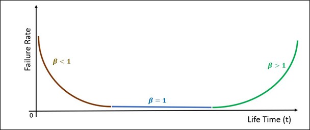
The shape parameter Beta in a Weibull distribution can indicate the failure evolution over time. It is also known as the Failure Rate function. The Beta value as defined below, will inform the analyst on the failure pattern and subsequent mitigative action required.
- Beta<1 is called the infant mortality section. This corresponds to early failures and a decreasing failure rate over time which in essence is undesirable. Infant mortality represents premature failures due to manufacturing defects or poor maintenance practices.
- Beta~1 is called the random failure section or useful life. This corresponds to the normal life of a component or asset where external factors influence its survival. Normally preventive maintenance or proactive repairs are not effective in this period due to the random nature of failures.
- Beta>1 is called the ageing or wear out section. This corresponds to the time in the life of a component where age related failures appear and increase over time. The use of the component over time will induce mechanical stresses leading to obsolescence. And an increase in repair frequency and subsequently cost.
Most assets have a “U shape” like life cycle known commonly as the Bathtub curve (Diagram 2). This is a combination of 3 Weibull distributions. All three beta value types highlighted above are represented in the curve. Note that the wear out phase (Beta >1) is somewhat the easiest phase to manage. It allows the asset manager to plan for impending failures or obsolescence.
Decision Pointer #2 – Component Optimal Replacement Time
If a Weibull distribution is used to model the life of an asset, we could use a Cost Optimization Process to determine when it is most cost effective to replace the entire asset. The more frequently we replace an asset (e.g. an automobile), or conduct any maintenance task, the higher the cost incurred. Yet the lesser the risk of failure. Conversely, the less frequent the replacement, the higher the risk of failures hence the potential increase in lost revenue and/or high unplanned repair costs. There is an optimal point combining cost, maintenance frequency and life characteristics which will indicate the optimal replacement time. The graphical output related to the optimization exercise is highlighted in Diagram 3 below. This is a very useful tool for asset managers in order to establish future maintenance budgets. Let alone reduce the risk of unplanned failures.

Decision Pointer #3 – Maintenance Strategy
Using the same concept as above in Decision Pointer #2, one can go a further in defining the correct Maintenance Strategy. For example, is an inspection or CBM task more cost effective than a replacement strategy for a component? An appropriate CBM task can be none invasive and more informative on the condition of a specific component. It can also be cheaper than an invasive maintenance task where equipment needs to be disassembled.

In the example above (Diagram 4), the Life Analysis Model has been built using a Weibull Distribution where Beta=1.6 and Eta=87.64 months. The optimization curves provide the following information:
- The optimized planned replacement interval is every 31 months,
- The optimized planned inspection interval is every 5 months.
The planned replacement optimal cost is higher than that of the planned inspection. Therefore, planned inspection is recommended.
Decision Pointer #4 – Conditional Reliability
Sometimes we have an asset running for some accumulated time and need some indication of what the future performance will be between today and a future date. Conditional Reliability is the probability of a system successfully completing another mission following the successful completion of a previous mission. In other words, if a system has survived to this date, what is the probability of it surviving a defined future interval? As a practical example, if I am an 80-year-old male and have survived to this day, what is the probability that I survive another 2 years?
This calculation is useful for short term risk analysis. For example, what are the risks incurred if the organization considers deferring the replacement of a critical asset?
Decision Pointer #5 – Block Diagram Modelling
A Reliability Block Diagram (RBD) is a graphical representation used to model the reliability of a system. It analyzes how different components work together to achieve overall system reliability. Or a desired throughput. It is also known as a Reliability, Availability and Maintainability (RAM) model. It shows the dependence relationships between the system and its components, allowing for the calculation of system overall reliability based on the reliability of individual subcomponents. The building blocks of the RBD are the life analysis models defined for each block in the entire system. This is illustrated in Diagram 5 below. The centrifugal pump (or system) is broken down into critical components and failure modes. Each component’s life analysis model will contribute to the overall life performance of the centrifugal pump.


Leave a Reply