
Introduction
A state variable is a parameter that is categorized into a countable number of defined states. Examples would include transmission gear states, PRNDL positions, ignition switch states, and others. Sometimes continuous variable, like pedal positions, may be binned into discrete states to be displayed as a histogram. State change timing is unpredictable since vehicle operation is highly variable. A way to deal with this data is Markov Analysis.
Markov Processes
First lets define a Markov process. Start with a transitions matrix to track states, table 1.
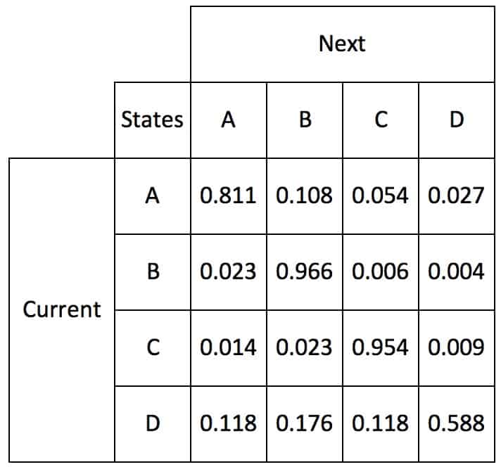
Table 1
In this example, if the current state is Xt at time t and Xt+1 at time t+1, then the cell that matches Xt and column Xt+1 is incremented by 1. In this example, if the Xt state is B and the Xt+1 state is D, then the B-D cell is incremented from 30 to 31. For telematics data, states don’t change often, but when they do, the transition is rapid. The diagonal cells accumulate the most one-second counts when due to infrequent cell changes. The off-diagonal cell counts represent the number of state changes because transitions occur rapidly.
If the cell counts in table 1 are added, the result is the total time in the telematics data. A way to model this process is as a Markov Chain graph is shown in figure 1.
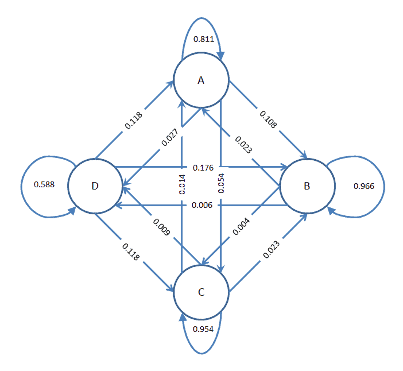
Figure 1
In figure 1, arrows show the transitions. The numbers associated with each arrow is the probability associated with a state transition. These are calculated with a Markov Transitions Matrix, table 1. For each row, the cells are added. Then the transition probabilities for each are calculated by dividing the cell counts by the row count total. These percentages are shown in table 2.
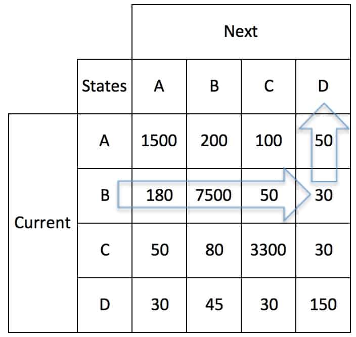
Table 2
The Markov Transitions Matrix defines the probability of state transitions. The highest probability is along the diagonal. The most likely state at time t+1 is the state at time t. For each row, the row-wise sum of probabilities of transitioning to all states sum to 1.
Transmission Data
Consider the 1 reading/second (1 Hz) CAN data for transmission usage. There is a current gear state at all times. The most common situation is the gear state doesn’t change, but a transition to another state can occur at any time. However, occasionally, there is a gear change resulting in incrementing an off diagonal cell. In a vehicle, the probability of a gearshift increases with time in response to vehicle usage or environmental factors. For the one-second telematics data, an 8-speed transmission Markov data table could look like.

Table 3
In table 3, the gear states are reverse, neutral and the gear number. The current state is the gear position at time t and the next state the gear position at time t+1. Again, the counts are stored in the cells. A bullet is shown to avoid the release of corporate information.
The cells contain 0 or an integer, the count of seconds. On the diagonal, the Current and Next gear states are the same so the cell contain the total operating time in the gear. A gear designer would be interested in the total operating time in a gear, as it is major factor in gear fatigue life calculations
Gear changes are stressful events that may result in failures. When the change occurs, the Current and Next gear states are different. The appropriate cell in the table is incremented by one. At the next time interval, if the state has not changed, the cell to increment is again on the diagonal. Therefore the off diagonal cells contain the gearshift counts.
The number of transitions into a gear is stressful events and of interest to gear designer and development engineers. In table 3, the transitions into a gear will be the sum of it’s column, less the diagonal cell from the column. When combined with torque and speed data, the result could be improved reliability tests.
Rain Flow Analysis Counts
A electronic failure modes may be caused by thermal cycling. Component specific cumulative damage models are used to analyze the damage created by the thermal cycles. An important factor for these models is the cycle count for each peak (maximum) and valley (minimum) temperature bin. A cycle counting method called rain flow analysis provides these cycle counts.
A graphic of the local environment thermal cycles near a module is show in figure 2.
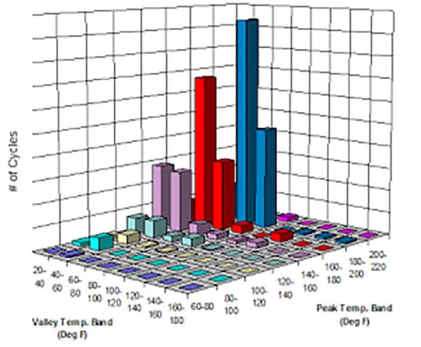
Figure 2
Figure 2 was published in “Accelerated Life Test – Simulation Integration”, by James McLeish, in the SAE Automotive Excellence, Spring, 2017. These thermal cycle counts provides a basis for modeling damage to the electronics.
In this analysis, the temperature bins were define with 20°C interval widths centered on -30°C, -10°C, 10°C…110°C, 120°C. This results in a large table that captures a vehicle’s thermal history over a period of time.
A comparison of the Markov approach to the cycle approach shows a 2:1 relationship, i.e., the Markov transitions are twice the rain flow counts.
The cycle count table is used to perform cumulative damage analysis for electronic components in a module. Again, this requires design knowledge for each component as well as the temperature rise from the local environment to the component in the assembly. The damage results for individual vehicle may be projected to 10 years of operation and analyzed statistically.
Pedal Strokes
An accelerator pedal assembly includes many mechanical parts and can wear out from excessive pedal usage. When the driver depresses the accelerator pedal, it results in a stroke. When the driver relaxes his foot, a spring causes the assembly to follow the driver’s foot in reverse stroke. Because the assembly is under stress, metal accumulate fatigue damage and bushings experience wear. An engineer needs to verify the assembly in durability tests.
The pedal positions are measured with a sensor as a voltage and communicated on the CAN bus. When the driver depresses the accelerator pedal, it produces an increase from some initial low voltage to a final higher voltage at the peak of the stroke. When the driver releases the accelerator pedal, the voltage drops to a low value at the end of the stroke.
To apply the Markov model, first define voltage intervals. The time series is analyzed to determine the initial and final voltage states, and the appropriate counter is incremented. Then the data was converted to a percentage and plotted, figure 3.
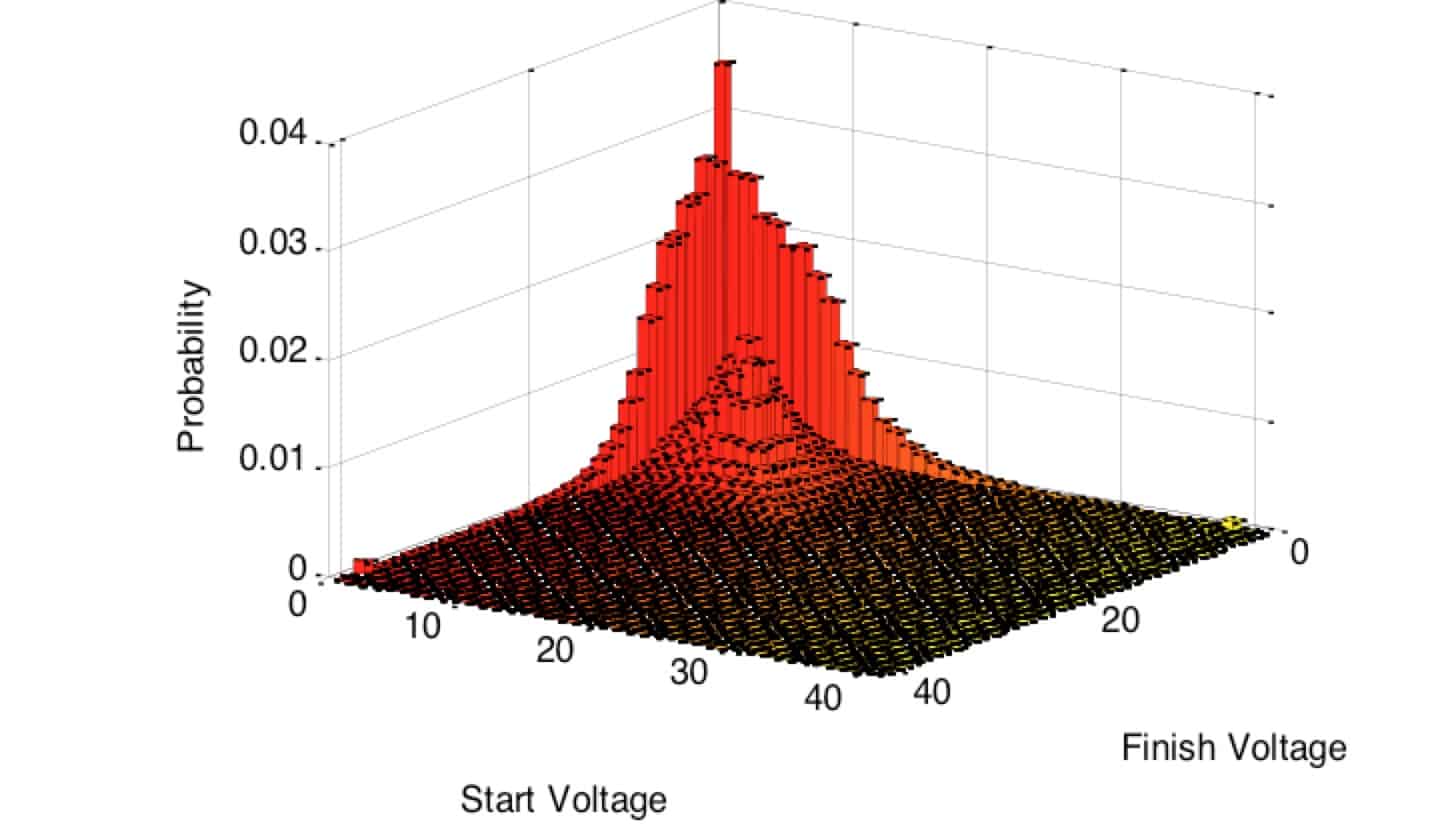
Figure 3
This figure shows a driving pattern where the pedal is at 0 voltage at either the start or end of many of the pedal strokes. This implies the driver was heavy footed. This pattern should be compared with other drivers to determine what is normal. Averaging over a fleet will produce a representative pattern for design and verification testing.
Since the wear and fatigue stresses are a function of motion, the off diagonal cycle counts are more important for the design engineer. The diagonal data represents stationary pedal situations where motion is very low so the wear and fatigue stresses are low.
Conclusion
Telematics data can be analyzed for components and subsystems by considering state changes. One may use Markov or cycle counting methods. The analysis provides design and test engineers with information that can be used to design and for verification testing.
Note
If you want to engage me on this or other topics, please contact me. I offer a free hour for the first contact to discuss your problem/concerns and to determine how I can help you. I want to help solve your design and manufacturing problems.
I have worked in Quality, Reliability, Applied Statistics, and Data Analytics over 30 years in design engineering and manufacturing. In Wayne State University, I taught at the graduate level. I also provided Minitab seminars to corporate clients, write articles, and have presented and written papers at SAE, ISSAT, and ASQ.
Dennis Craggs, Consultant
Quality, Reliability and Analytics Services, LLC
810-964-1529
dlcraggs@me.com
 Ask a question or send along a comment.
Please login to view and use the contact form.
Leave a Reply