The operating characteristic curve is used to understand lot sampling plan. It graphically provides a relationship between the unknown lot’s defect rate (or total) and the probability of the specific sampling plan to accept the lot. Very good plans discriminate between good and bad lots. Poor plans may accept bad lots or reject good lots to easily.
There are three methods to calculate the values of the OC curve, and in this short note we will use the hypergeometric distribution and consider the lot effect of changing the sample size drawn from the lot.
The hypergeometric distribution is described here.
In this example we have 500 units per lot and using the ANSI/ASQ Z1.4-2008 Sampling Procedures and Tables for Inspection by Attributes S-3 inspection level and single sampling plan, we draw eight samples. The acceptance is with no defects in the sample, r=0. The rejection of the lot is with one defect or more in the sample, c=1.
If I have the capability to draw five more samples for a total of 13, how would that change the ability of the sampling plan to accept lots with better than 1.5% defect rate and reject those with higher defect rates?
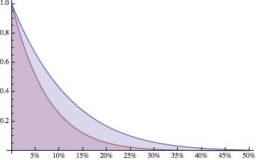
This plot is for 8 and 13 samples drawn from a lot of 500. The top curve is eight samples, and the lower curve is for 13 samples. For a lot with 1.5% defects the Pa=80.9% down from 87.8% with eight samples. Almost 7 points are more likely to find a defect in the sample and reject the lot. Y-axis is Probability of Accepting the Lot, x-axis is lot percent defective.
If the lot has 10% of units defective, the 13 samples are about 25% likely to accept the lot, whereas the 8 sample draw is roughly 45% likely to accept. Of course, more samples provides more information about the unknown characteristics of the lot. It always is a balance between cost of sampling and testing a lot and the expense of accepting a lot with some unacceptable number of defects. The OC curve provides one way to understanding and makes the final decision about a sampling plan.
Back to the calculation for a moment, above we calculated the probability of accepting the lot, Pa when the lot defect rate is 1.5%. Here is the formula and calculation.
$$ \large\displaystyle P(x,N,n,m)=\frac{\left( \begin{array}{l}m\\x\end{array} \right)\left( \begin{array}{l}N-m\\n-x\end{array} \right)}{\left( \begin{array}{l}N\\n\end{array} \right)}$$
This calculates the probability of exactly x successes in a sample of n taken from a population of N which contains m successes. For this problem we are defining the test failure as a success and we’re interested in the chance that a sample of 8, n, taken from the lot of 500, N, which has an expected total number of ‘successes’ of 7.5 (use integers in the formula, 8 in this case), m, would result in exactly 0, x, ‘successes’.
$$ \large\displaystyle P(0,500,8,8)=\frac{\left( \begin{array}{l}8\\0\end{array} \right)\left( \begin{array}{l}500-8\\8-0\end{array} \right)}{\left( \begin{array}{l}500\\8\end{array} \right)}=0.875$$
The calculation results in a probability of having exactly 0 ‘successes’ is 0.875.
And, repeat the same calculation for a sample of 13 from the same lot to find Pa=80.9.
To create the curves, repeat the calculations for each point along the x-axis which is the lot percent defective. For the formula, we need to calculate the number of good and bad items in the lot, which should not be too difficult.
Related:
OC Curve with Binomial Method (article)
How to read an OC curve (article)
Sequential Sampling by Attributes (article)

 Ask a question or send along a comment.
Please login to view and use the contact form.
Leave a Reply