Process Capability Analysis II – Percent Defective Estimates

Introduction

In my prior article, Process Capability I – Overview and Indices, the process capability concept was defined for prototype samples and serial production. The data is assumed to be normally distributed and P_p, P_pk, C_p, and C_pk indices were defined. Its application to one-sided and two-sided tolerances was discussed. This article provides methods to estimate the percent defective.

The Data

The engineering tolerance for a critical characteristic is 10±0.2. So the lower specification limit (LSL) is 9.8 and the upper specification limit (USL) is 10.2. A sample of 30 parts provided measurements of the critical characteristic. The sample mean ($-\bar{x}-$) was 9.951 and the sample standard deviation (s) was 0.1825.

Normality Assessment

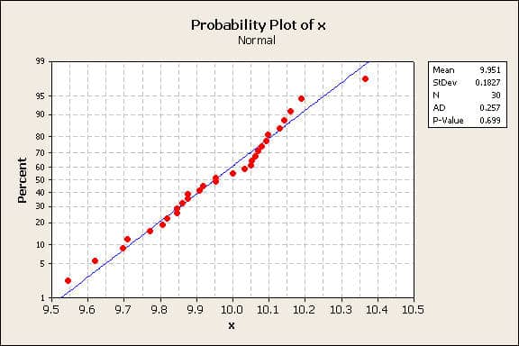
A basic PCA assumption is that the data is normally distributed. The 30 measurements were analyzed for normality. Many software programs support this type of analysis. A Minitab probability plot, figure 1, shows the data conforms to a normal distribution with a 0.699 goodness of fit. Since this is not a rare event, the hypothesis that the data is normally distributed can’t be rejected.

Figure 1

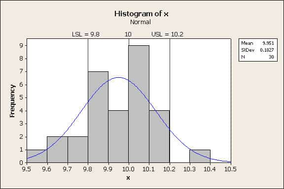
To visualize the data, a plot showing the data histogram, the best-fit normal distribution, and the engineering tolerances was created, figure 2.

Figure 2

While the mean is contained between the specification limits, the process variation is too large for the tails of the curve to be contained. The area under the tails of the normal distribution is so large that the probability of parts being manufactured outside of the tolerance limits is high. So how are the probabilities calculated?

Probability Calculations

The probabilities are the area under the distribution. Consider the case where the probability density is f(x) and we want to solve for the probability of events between x₁ and x₂, equation 1.

$$P({x_1}<x<{x_2})=\int_{z_1}^{z_2}{f(x)dx}$$

(1)

A similar form is the cumulative probability for any X value is the area from $-{-\infty}-$ to X, equation 2.

$$P(X)=\int_{-\infty}^{X}f(x)dx$$

(2)

Here lower case x is a dummy variable for the integration and f(x) is the probability density function. If f(x) can be integrated, then an equation that provides an exact solution can be determined.

If the data is normally distributed, then f(x) is

$$f(x)=\frac{1}{\sqrt{2\pi}\sigma}e^{-(x-\mu)^2/2\sigma^2}$$

(3)

Equation 3 is simplified by letting z = (x-µ)/σ yielding the standard normal, equation 4.

$$f(z)=\frac{1}{\sqrt{2\pi}}e^{-z^2/2}$$

(4)

The normal equation can’t be integrated so numerical methods are required.  Fortunately, tables for the cumulative standard normal distribution have been compiled. Also, software like Excel, Minitab, SAS and JMP contain functions that calculate cumulative normal probabilities.

Statistics Tables

Statistical tables may be used to estimate cumulative probabilities. These tables are found in statistics textbooks, but the tables can be organized in several different ways. Let’s assumes a table of the cumulative standard normal tabulated for z values from -6 to +6. To calculate the lower tail cumulative probability, first calculate the z₁ value for the LSL, equation 5.

$$z_1=\frac{LSL-\mu}{\sigma}$$

(5)

In our example, z₁ = (9.8-9.951)/0.1825 = -0.827. This expresses the LSL in multiples of σ. Looking up the z value from a standard normal cumulative distribution table provides the lower tail probability of 0.204, or about 20% in the lower tail. Interpolation between table values is generally required.

A similar process is required for the upper tail. The USL is converted to multiples of $-\sigma-$, equation 6.

$$z_2=\frac{USL-\mu}{\sigma}$$

(6)

In our example, z₂ = (10.2-9.951)/0.1825 = 1.364. Looking up the value provides the cumulative distribution of 0.914 for z₂, which is subtracted from 1 to determine the upper tail probability of 0.086, or 8.6%

Excel

Modern computer software provides tools that are easier to use. For example, Excel provides the function norm.dist that supports cumulative normal probability calculations. The function requires an x value; the mean μ; the standard deviation σ; and a logical argument with a value of true, equation 7.

$$P(X{\leq}x)=norm.dist(x,\mu,\sigma,true)$$

(7)

Here X is the normal random variable. To calculate the lower tail probability, substitute LSL for x, equation 8.

$$P(X{\leq}LSL)=norm.dist(LSL,\mu,\sigma,true)$$

(8)

For the example data, the Excel function yielded 0.204, conforming to the table results.

For the upper tail, the cumulative probability of the USL is subtracted from 1, equation 9.

$$P(X>USL)=1-P(X{\leq}USL)=1-norm.dist(USL,\mu,\sigma,true)$$

(9)

For the upper tail, the Excel function yielded 8.6% in the upper tail.

Tail Probabilities

The normal distribution in Figure 1 was not centered, so the lower and upper tail probabilities were unequal. If the distribution is centered between the engineering specification limits, equations 8 and 9 yield the same tail probabilities, because the normal distribution is symmetric.

When the tolerance limit is two sided, both the lower and upper tail probabilities need to be calculated and then added to determine the total non-conforming probability. When the tolerance limit is one-sided, only one tail probability needs to be calculated. For example, if there is only a LSL, then equation 8 is used to calculate the lower tail probability. If there is only an USL, then equation 9 is used to calculate the upper tail probability.

PCA Software

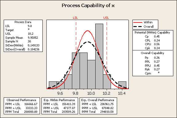
Minitab, JMP, and Matlab software provide support for Process Capability Analysis. Minitab was chosen for an example. Minitab is general-purpose statistical software package that provides a nice graphical summary of process capability, figure 3.

Figure 3

Figure 3 contains a lot of information useful for a PCA assessment.

• A graphic containing a histogram of the data; the LSL and USL; and an “Overall” and “within” probability distribution. The “Overall” uses a standard deviation calculated assuming the data is one group. The “within” method uses different statistics for subgroups.
• In the upper left box, the specifications and data statistics are summarized.
• In the right boxes, Potential and Capability indices are summarized. The Potential indices are the P indices. The Capability indices are the C-indices.
• At the bottom are boxes that summarize observed, and expected performances. The predictions are in terms of PPM, not probability.

For more detail, Minitab help provides more detailed answers, beyond the scope of this article.

Conclusions

• PCA data may be used to determine the percentage defectives.
• Tables of the standard normal distribution cumulative probabilities vs. z may be used to estimate the lower and upper tail probabilities.
• Excel functions may be use to directly calculate the lower and upper tail probabilities.
• Several major general purpose statistical software packages support Process Capability Analysis.

Next

The next article in the Process Capability series discusses the importance of maintaining a relatively high Cp index to reduce the percent manufacturing defects: Cp vs Percent Defectives.

Note

If you want to engage me as a consultant or trainer on this or other topics, please contact me. I have worked in Quality, Reliability, Applied Statistics, and Data Analytics over 30 years in design engineering and manufacturing. In the university, I taught at the graduate level. Also, I provide Minitab seminars to corporate clients, write articles, and have presented and written papers at SAE, ISSAT, and ASQ. I want to assist you.

Dennis Craggs, Consultant
Quality, Reliability and Analytics Services
810-964-1529
dlcraggs@me.com