
Introduction
Reliability Engineering analytics come with graphs and visual representations providing the analyst with various types of key information. Some graphs are more popular than others. This article highlights the 4 main graphs used in Reliability Engineering Analysis.
They are Reliability, Probability of Failure, Probability Density and Failure Rate. Less common types are not covered here. Such as Contour Plots. The basis of the graphs in this article is the Weibull Distribution. In other words, all the graphs derive from this very popular distribution. The same concepts applies to other distributions.
Reliability Academic Definition
The concept of Reliability is often misused, misunderstood, and misinterpreted. Reliability in its academic root, is defined as the probability that a system will perform its intended function in a specified mission time and within specific process conditions. So, it is in essence a Probability.
The time variable is crucial in understanding the reliability of a system. Reliability is the Probability of Success. And 1 minus the Probability of Failure.
$$ \displaystyle \large R\left(t\right) = 1 – F\left(t\right) \:\:\:\: (where \: F = Failure \: Probability) (1) $$Let us apply this concept to that of a Roller Bearing. The life analysis of a Roller Bearing population is modelled by a Weibull Distribution. A question that could be asked is (2):
- What is the Reliability of a newly installed bearing for a year, provided it is operating within ideal specification parameters?
- Or… what is the probability that the bearing will last a year without an unplanned failure within those same conditions?
Reliability Functions and Graphs
Using Equation (1) above, we have two functions (R(t) and F(t)). Hence, we will have two graphs for the bearing as shown below.
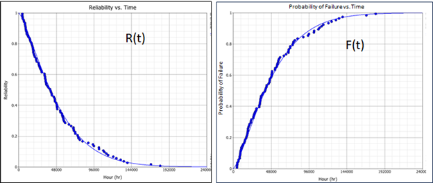
By nature of the mathematical equations (1), the two graphs are mirror images. Question 2 above can be graphically answered such as: R(t=8,760 hours) = 91%. In other words, the bearing has a 9 % chance of failure after one year of operation.
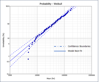
F(t) has multiple names. It is known as the Cumulative Density Function or the Unreliability Function. And is a mathematical integration of the Probability Density Function covered below. The Weibull distribution has unique and highly useful particularities. Its derived Probability of Failure function can be turned into a straight line through logarithmic transformation. Graph 2 below illustrates this transformation. There are a lots of visual advantages to this graph including changes in inflection (e.g. Doglegs) as well as the ability to evaluate the model validity using Confidence Boundaries.
Probability Density Functions (PDF) and Graphs
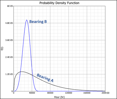
The Probability Density function is a normalized Frequency Graph. The integrated area under the graph is equal to 1. The PDF graph provides the analyst with an overview of the data layout. Especially relating to the scatter or variability of data. Graph 3 below shows PDF curves for two Roller Bearing types. Bearing A has a larger variability in terms of its time to failure. This suggests that Bearing B will have a more precise range of time to failure around the peak (mode) of 30,000 hours of operation.
Failure Rate Functions (PDF) and Graphs
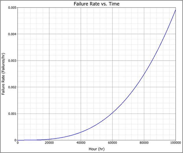
The Failure Rate function highlights the “speed” of failure over time. Typically, though not always, age will cause accelerated degradation in components or assets. For example, an ageing automobile in continuous use, will see more frequents failures over time until it is no longer economically viable to keep it. Its Failure Rate will increase over time.
The patterns associated with the Failure Rate curve indicate the Failure nature. In the case of our initial bearing B above, because its Beta Parameter is more than 1, it will show an increase in Failure Rate over time (Graph 4). Signaling wear out and imminent loss of function.
One of the best-known concepts and subsequent graphical representation relating to Failure Rate is the Bathtub curve. It is a combination of 3 Failures Rate curves with 3 Beta values as follows.
- Beta less than 1, representing infant mortality or early failures,
- Beta equal to 1 representing random failures,
- Beta more than 1, representing ageing or wear out failures.
Graph 5 below illustrates a theoretical example of a Bathtub curve.

In summary, graphical representations in Reliability Engineering are precise and can be very informative to the analyst. However each graphical representation type relates to a specific mathematical function.

Leave a Reply