This is hopefully completely a review. The mastery of basic statistical terms is important as many of the questions on the CRE are statistical in nature and rely on your understanding the terms. Let’s simply review the terms, and do let me know if you have any questions.
Let’s take a random sample from a population. Given a
classroom of adults in a classroom as the population I’ll assign each person a number, from one to thirty (30 folks in the class). Now, using a trusted random number generator select 5 random numbers without replacement from the sequence 1 to 30. For sake of argument, let’s say these five are
3, 6, 12, 17 and 21.
So, those students with these assigned numbers, please stand forward for height measurement. And, in inches, these turn out to be
61”, 64”, 65”, 66”, and 73”.
First, do these numbers appear to be random?
While it is possible for both the random numbers pulled from a list are in order, it’s rare. Also, the heights, unless the group was standing in height order when assigned their numbers, also a rare occurance, also. Possible, yet not likely. The same exercise could easily occur without the sequences being in order.
Sample – the group of five pulled from the population and we can use the sample to understand the larger population without measuring the full population.
Population – the defined group, in this case, the classroom of 30 students. Populations can be the production of iPods, people in New Zealand, cars in India, etc.
Random – no particular order or pattern. For example, not every fifth person, or a production product taken each hour. A truly random sample takes some thought and work to make happen.
Simple random sample – is a selection of items from a population such that any item in the population has an equal chance to be selected into the sample.
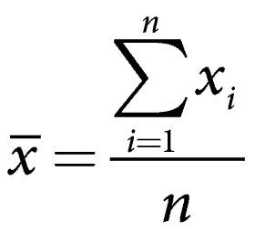
Now that we have a sample, what is the estimated average height of all students in the room? We can calculate
where,
x̅ = the mean
∑ = is the summation operation
x = is each number, the subscript i is an index for each number
n = is the number of samples, or sample size.
The x̅ is a statistic used to estimate the unknown population parameter, μ.
A statistic is some data value calculated based on a sample that provides an estimate about the population.
A parameter is a value describing some characteristic about the population.
In the simple example about heights, the x̅ is the mean value estimating the population mean, μ.
Mean is the sum of all the values divided by the number of items. For the sample of heights, we have
The mean is one way to describe the central tendency measure. There are two others, median and mode.
The mean is the center of gravity of the data. Using the analogy that each data point has the same mass the same and are spaced along a sequence of equally spaced number (say a ruler) from 61 to 73, one could find the balance point of the beam at the mean value point. You could put your finger under the ruler and the balance point would be 65.8 along the ruler.
Another advantage of the mean calculation is it uses all the data, yet a disadvantage is one either very small or large (significantly different than the other data values) will distort where the bulk of the data occurs. To calculate the mean one does not need to sort the data, as in the median. A couple of disadvantages include the calculation may take longer to accomplish than the median or mode, and it may result in a value that is not the same as any data value.
The median is the midpoint of the data. Sort the data and select the data point in the middle. For an odd number of data points, as in our simple heights example, it’s the middle point in the ordered sequence. I this case it’s 65. For an even number of items, it’s the average of the two middle values. The median provides information on where most of the data exists, other than sorting takes very little calculation and is insensitive to extreme values.
The last advantage is why home values of recent sales are often reported as a median. The data does take a sorting to find the median, and in some datasets the extreme values may be important. Medians cannot be averaged, like means to find a combined distribution statistic. And the median will have more variation than a mean when taking repeated samples from the population.
The mode is the most frequent data value. In this case, there are five different values. Therefore, mode either doesn’t exist or is any of the points, in either case, it’s not very useful. In the case where there are two people in the sample with 64 as their height, and all the others were unique, then the mode would be 64.
The mode is very easy to determine, it’s just the data value that occurs the most, thus only simple counting. It is not influenced by extreme values and it will be an actual value of one of the data points (if it exists) and is easy to see in a histogram plot (it’s the high point – more on histograms later).
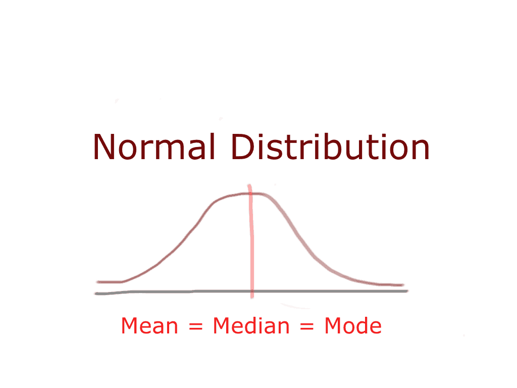
To wrap up this short review of terms, consider a normal distribution. It is a continuous distribution, meaning it contains infinite (variable) data points that come from a continuous measurement scale, like heights. Other continuous distribution include Weibull or log normal. For the normal curve the mean, median and mode are the same.
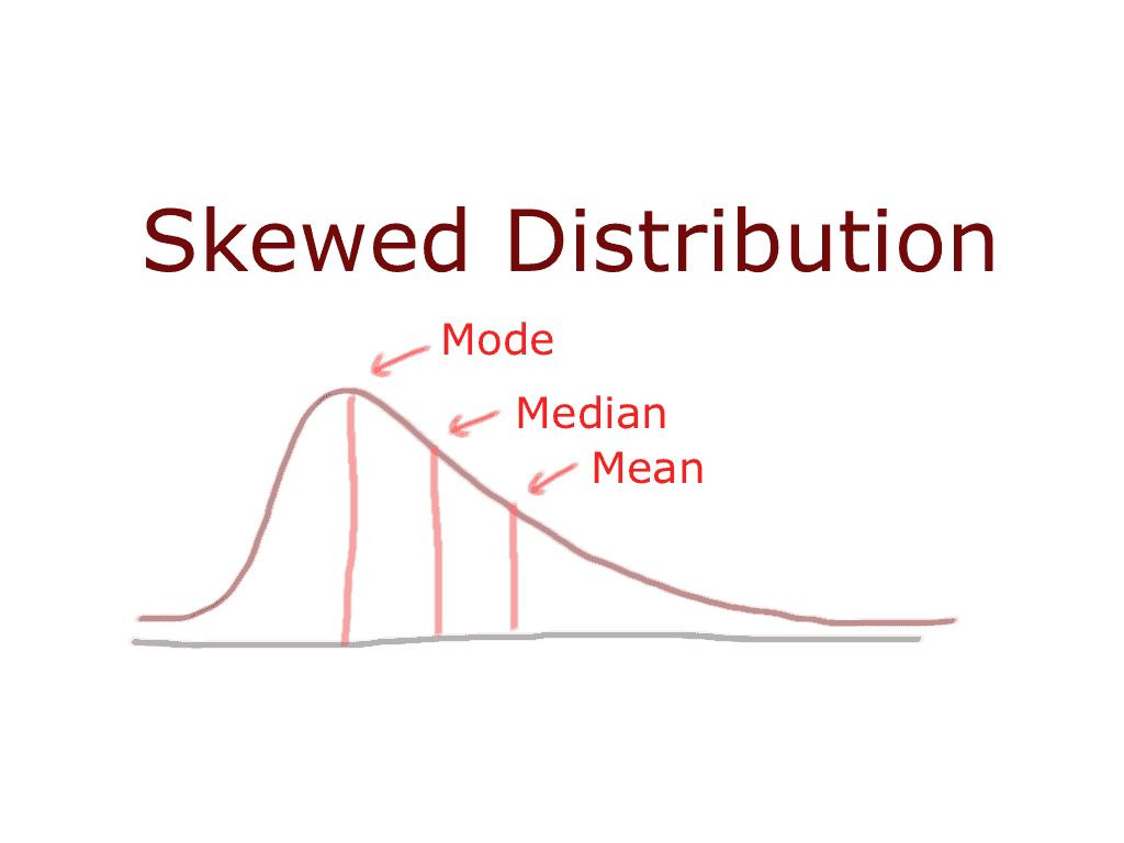
 For a skewed distribution, meaning the data appears stretched out on one side or the other, the mode is the most common data value, median is the middle point, and mean is the center of gravity of the data. More of skewness and distributions later.
  Note: I’m playing with a few ways to draw and get the image or formula to appear… maybe be some variation as I sort these tools out.
Related:
Statistical Confidence (article)
Statistical Terms about Variation (article)
Variance (article)


 Ask a question or send along a comment.
Please login to view and use the contact form.
Excellent work! I really appreciate your help and support!