In probability theory and statistics, the Weibull distribution is a continuous probability distribution. It models a broad range of random variables. Largely in the nature of a time to failure or time between events. It addresses mechanical or structural failures in the field of Reliability Engineering. By nature, the Weibull distribution provides a lot of information such as aging characteristics or expected asset lifetime. One of its most common outputs is the Bathtub Curve.
It is not very common to see a Weibull distribution used to analyze production output. By production output, we mean the daily output of a plant, factory or production line. It is a top-down approach and the production plant treated as a “black box”. Meaning that we do not really focus on the details inside the black box. The Barringer Process Reliability (BPR) methodology can analyze production performance appropriately. It is based on the 2 parameter Weibull distribution. The two parameters being the shape and scale parameters.
On the contrary, Traditional Reliability analysis is based on the details inside the “black box”. In other words, it is a bottoms up analysis.
Traditional Reliability analysis using the Weibull Distribution.
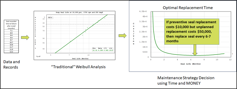
As mentioned above, Traditional Reliability analysis goes into the “guts” of the asset. This requires a lot of records and information. The example in Diagram 1 below illustrates the analysis of a bearing population failure. As well as the subsequent potential action required. The bearing time to failure is sourced from the Computer Maintenance Management System (CMMS). The Weibull statistical model represents a typical bearing life pattern. When financials and life models are combined, the optimal bearing replacement time is defined. As shown in Diagram 1 below, it lies between 6 and 7 months.

The model can provide various additional information. We have listed only the optimal replacement interval calculation. However, the point of the matter is that each and every component or asset similar to a bearing needs to be studied in detail. This makes analysis complex and time consuming.
BPR Analysis
Contrary to the Traditional Reliability analysis highlighted above, Barringer Process Reliability only requires Daily Production records. For example, for a brewery bottling line, in a 365 day period, we would only need the daily total hectoliters of beer bottled.
BPR is a production analysis methodology, invented by Paul Barringer. It is a simple yet powerful method allowing senior leaders to assess and quantify the performance of their production plant. They would achieve this using only simple graphics and a set of key performance indicators. The BPR output can be viewed on one side of a single sheet of paper. That is why it is also called “the factory on a page” analysis.
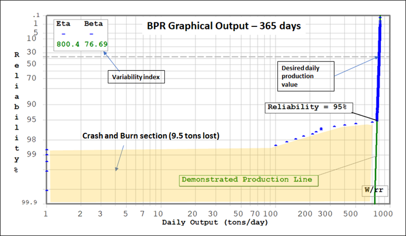
The underlying mathematical concept for BPR is the Weibull Statistical Distribution. Daily production data randomness can be modeled using a Weibull distribution. The Weibull distribution allows for straight lines in logarithmic plots. A unique property attributed to this distribution. As well as quantifying production performance, BPR has visual properties as illustrated below in Diagram 2.

BPR does not go into the details of low production performance. It remains at a high level (the 10,000ft overview). However, it is still able to quantify production losses as well as opportunities for revenue enhancements. It also has the unique capability of measuring variability in production output using the shape parameter (beta). Diagram 3 below provides a typical graphical output of a BPR analysis.

In summary, Both BPR and Tradition Reliability methods are extremely useful to predict and manage asset performance. When requiring detailed information such a spare-parts stocking requirements or individual maintenance strategies, Traditional Reliability is the tool of choice. BPR stands out as a management tool. It provides strategic information without going into the weeds of problems. Traditional Reliability deals with the weeds.
 Ask a question or send along a comment.
Please login to view and use the contact form.
Leave a Reply