A continuous distribution is useful for modeling time to failure data. For reliability practitioners, the Weibull distribution is a versatile and powerful tool. I often fit a Weibull when first confronted with a life dataset, as it provides a reasonable fit given the flexibility provided by the distributions parameters.
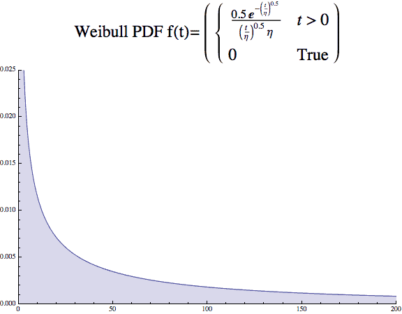
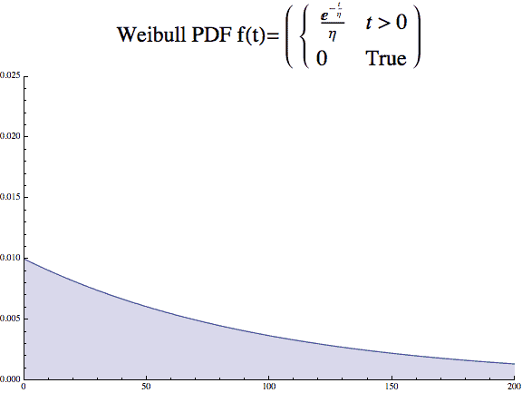
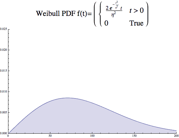
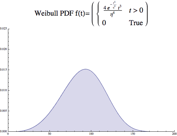
The beta, β, value is called the shape parameter and describes the shape of the distribution, think histogram. It ranges from describing data that show a decreasing failure rate over time, β <1, to a with an increasing failure rate, β >1. When β =1, the Weibull distribution exactly equals an Exponential distribution and describes a constant failure rate.
Here is the formula for the Weibull Distribution probability density function. The PDF is like a histogram as it shows the relative rate of failure over time.
$$ \large\displaystyle \begin{array}{l}f(x)=\frac{\beta }{\eta }{{\left( \frac{x-\gamma }{\eta } \right)}^{\beta -1}}{{e}^{-{{\left( \frac{x-\gamma }{\eta } \right)}^{\beta }}}},\text{ for }x\ge \gamma \\f(x)=0,\text{ for }x\lt \gamma \end{array}$$
A few plots will show the impact the β value has on the look of the distribution. The x axis is time, and y axis the probability density.
And while the static images are common, and many would overlay the images onto one plot.
There is a lot more to the Weibull distribution, and I’ll be writing more soon. In the meantime here are two references that are worth reviewing.
Webb, Willie M., Andrew N. O’Connor, Mohammad Modarres, and Ali Mosleh. “Probability Distributions Used in Reliability Engineering.” In Probability Distributions Used in Reliability Engineering. College Park, Maryland: Center for Risk and Reliability.
Related:
Calculate Weibull Mean and Variance (article)
The Normal Distribution (article)
Reading CDF plots (article)


 Ask a question or send along a comment.
Please login to view and use the contact form.
Leave a Reply