
Imagine product or part lifetime as the service time in a self-service system. Suppose you could observe periodic input and output counts of that self-service system, without identifying individual service times. How would you estimate the service time distribution without following individual products or parts from input to output? The maximum likelihood reliability estimator for an M/G/Infinity self-service-time distribution function from “ships” (inputs) and “returns” (outputs) counts also works for nonstationary arrival process M(t)/G/Infinity self-service systems, under a condition! A constant or increasing arrival (inputs or ships) rate satisfies the condition. If you identify returns by failure mode then you could estimate make nonparametric estimates of field reliability by failure mode and quantify reliability growth, without life data, if the condition is satisfied.
Failure?
Recently a friend sent me his annual sales and returns.
Table 1. Nevada table of ships (sales) and returns (sums in bottom row)
| Year | Sales | 2020 | 2021 | 2022 | 2023 | 2024 | 2025 |
| 2020 | 393 | ||||||
| 2021 | 502 | ||||||
| 2022 | 592 | ||||||
| 2023 | 141 | ||||||
| 2024 | 0 | ||||||
| 2025 | 0 | ||||||
| Returns | 14 | 9 | 11 | 12 | 3 | 5 |
I computed the nonparametric reliability estimate using my 30+ year old spreadsheet, https://docs.google.com/spreadsheets/d/1fb_pjwygp_2CUeayNEV4PAX6wyR8sdWqPr76qeJ_n4I/edit?gid=0#gid=0/.
Table 2. Nonparametric maximum likelihood reliability estimators from successively earlier cohorts
| Age, years | All cohorts | -2025 | -‘24&’25 | Etc. | Etc. | 2020 |
| 1 | 0.9771 | 0.9771 | 0.9771 | 0.9771 | 0.9743 | 0.9644 |
| 2 | 0.9771 | 0.9771 | 0.9771 | 0.9771 | 0.9743 | |
| 3 | 0.9771 | 0.9771 | 0.9771 | 0.9771 | ||
| 4 | 0.9149 | 0.9149 | 0.9149 | |||
| 5 | 0.8936 | 0.8936 | ||||
| 6 | 0.8582 |
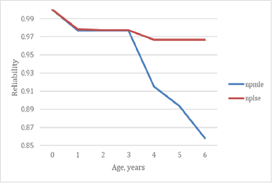
Because the sales were zero in 2024 and 2025, I became suspicious that the PAV (Penalize Adjacent Values) algorithm for nonparametric maximum likelihood estimator (npmle) of a nondecreasing cumulative distribution function G(s) might fail [Marshall and Proschan]. So I also computed the least-squares reliability estimator (nplse). (Thanks to Dick Mensing for suggesting this in 1991, https://accendoreliability.com/uncertainty-in-population-estimates/#more-503100/.) Notice how the reliability npmle goes nuts in ages 4, 5, and 6? That’s because a condition for the PAV algorithm is violated.
The npmle is valid if E[λ(t-S)]=∫λ(t-s)dG(s), integrated over s=1,2,…,t, is non-decreasing [George 1994]. Table 3 uses the nplse probability density function estimate, not that from the npmle, because the PAV algorithm produces non-decreasing E[λ(t-S)], whether the reliability estimate is valid or not.
Table 3. Condition for validity of PAV npmle algorithm: entries λ(t-s) are the ships, E[λ(t-S)] is approximated by ∑p(s)*λ(t-s), s=1,2,..,t where p(s)=G(s+1)-G(s).
| t | λ(t-s) | Etc. | Etc. | Etc. | Etc. | Etc. | p(s) | E[λ(t-S)] | NonDecreasing? |
| 1 | 393 | 0.02 | 8.68 | Eh? | |||||
| 2 | 502 | 393 | 0.00 | 9.03 | TRUE | ||||
| 3 | 592 | 502 | 393 | 0 | 13.5 | TRUE | |||
| 4 | 141 | 592 | 502 | 393 | 0.01 | 7.8 | FALSE | ||
| 5 | 0 | 141 | 592 | 502 | 393 | 0 | 5.5 | FALSE | |
| 6 | 0 | 0 | 141 | 592 | 502 | 393 | 0 | 6.33 | TRUE |
Reliability Estimation Without Life Data?
[The following article dates from 1994, unpublished.]
Except for high-cost or repairable products or parts, there is little incentive to record when returns or failures were shipped, so there is no time-to-return data from which to estimate reliability. Since 21 CFR Part 821, “Medical Device Tracking Requirements”, pacemakers have been tracked by serial number from implant to failure. Medtronic used to advertise periodic pacemaker sales and failure counts and their reliability estimates from their lifetime data. I made nonparametric reliability estimates from their periodic pacemaker sales and failure counts. Our reliability estimates agreed, and I sent them to Medtronic. Medtronic quit advertising periodic sales and failure counts from their pacemaker lifetime data!
Product lives may be regarded as service times of an M/G/Infinity self-service system. (“M” means inputs are a stationary Poisson process with service time distribution G(t).) System inputs are “ships”: product sales, installations, or shipments, by accounting interval. System outputs are “returns”: complaints, failures, repairs, replacements, spares ships or returns.
Larry Baxter derived a reliability function estimator from ships and renewals data, when all the ships occurred at the start of reporting. Unfortunately ships occur every month, and returns come back without a clue about how old they are.
Ships and returns counts provide statistically sufficient data to estimate products’ and parts’ reliability functions. A reliability function is one minus the service-time distribution function G(t) of an M/G/Infinity self-service system, because ships “serve” for a random time [George and Agrawal].
The output from an M/G/Infinity service system is a Poisson process with mean rate λG(t) where λ is the Poisson mean input rate [Mirasol]. The Poisson output mean rate λG(t) is analogous to the failure rate function of a time-to-failure random variable. Ulf Grenander and later Albert Marshall and Frank Proschan derived the Pool Adjacent Violators (PAV) nonparametric maximum likelihood estimator (npmle) of an nondecreasing failure rate function. The npmle of λG(t) gives the npmle of G(t) by dividing λG(t) by the input rate λ, because, under reasonable conditions, a function of an npmle is also an npmle. Reality may violate conditions to represent returns as output from a M/G/Infinity system.
What if Ships Process is Not Stationary?
Nonparametric maximum likelihood reliability function estimates, from ships and returns counts population data, derivable from data required by generally accepted accounting principles, are desirable for their properties and require no unwarranted distribution assumptions. They could be valid even if the input Poisson process rate λ(t) is nonstationary.
Theorem 1 of the article by Eick, Massey and Whitt says, “The departure process (of a nonstationary M(t)/G/Infinity service system) is a Poisson process with time dependent output rate δ(t)=E[λ(t-S)].” S is the service-time random variable, the expected value E[λ(t-S)] is ∫λ(t-s)dG(s), integrated from s=0 to t for periods t=1,2,…, and λ(t-S) is the ships input rate at time t-S. G(s) is the cumulative distribution function of service time S. If E[λ(t-S)] is nondecreasing, then the PAV nonparametric maximum likelihood estimator may be used to estimate reliability 1-G(s).
For example, suppose the Poisson ships rate is a constant λ. Then, E[λ(t-S)]=∫λdG(s)=λG(t)) and is nondecreasing because G(t) is a distribution function, nondecreasing in age t. For another example, suppose the Poisson rate λ(t) is a linearly increasing function, λo+λt, for t ≥ 0. Then, E[λ(t-S)] = ∫(λo+λ(t-s))dG(s) = λ(λo+λG(t)) and is also nondecreasing.
The npmle of E[λ(t-S)] puts mass at a subset of M(t)/G/Infinity departure times (return times in the reliability context). Those masses may be solved for the discrete npmle of the probability density function g(t). The npmle of E[λ(t-S)] with linearly increasing λ(t) is the npmle of λo +λ[G(t) – G(0) – ∑ug(u)], where the sum from u>0 to t runs over the set of return times, u, at which the npmle of E[λ(t-S)] puts mass. This discrete function can be solved for G(t) at jumps. The npmle of G(t) is constant elsewhere.
Suppose the first return occurs at time t1>0 and the npmle puts mass g(t1) at t1. Then the npmle of G(0) is 0 and the npmle of g(t1) is (g(t1)-λo)/(λ(λ-t1)) if nonnegative. Remaining values of g(u) may be solved recursively for values of u where the npmle puts mass.
An Example of Grouped Data
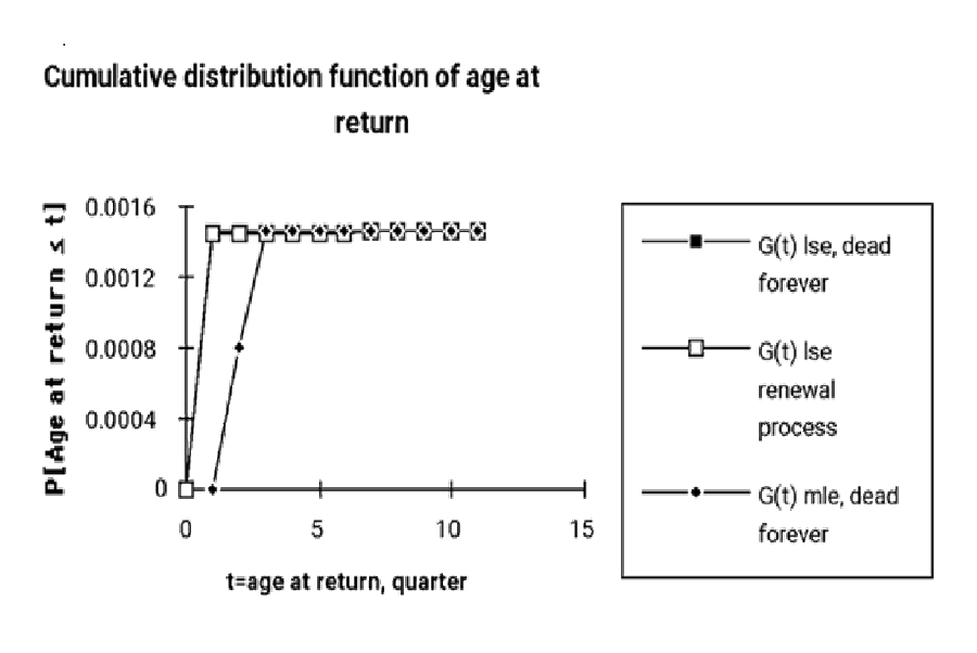
Table 4 shows the numbers of ships and returns by quarter for a product. Figure 2 shows the npmle and nonparametric least squares estimates (nplse) [George 2008] of the cumulative distribution function G(t) of ages-at-returns. There is not enough data to test whether the ships process is nonstationary Poisson. The condition for using the npmle with a nonstationary Poisson input is satisfied for all observed times. Table 5 lists increasing values of E[λ(t-S)].
Nonparametric least squares estimators (nplse) are computed under two assumptions: returns are from dead forever products or products that undergo renewal. Both estimators agree on G(t) after the third quarter (figure 2). The nplse puts all failure probability in the first quarter, and the npmle divided it between the third and fourth quarter.
Suppose the input rate λ(t) doesn’t keep up with the output rate, so ships < returns in a period. This violates the conditions for the maximum likelihood estimator [George 1993]. The returns may be a renewal or other kind of replacement process and need a different model of ships and returns such as a renewal process shown in figure 2 [Tortorella, George 2008].
Table 4. Ships and returns data. E[λ(t-S)] should be nondecreasing for a valid npmle.
| Quarter | Ships | Returns | E[λ(t-S)] |
| 1 | 892 | 0 | 0 |
| 2 | 64537 | 52 | 0 |
| 3 | 352133 | 937 | 0.7187 |
| 4 | 851677 | 2826 | 52.58 |
| 5 | 1452959 | 3913 | 325.6 |
| 6 | 2469820 | 4175 | 914.6 |
| 7 | 3815927 | 7975 | 1723 |
| 8 | 5288164 | 9326 | 2932 |
| 9 | 6837147 | 6962 | 4676 |
| 10 | 8268514 | 9436 | 6735 |
| 11 | 6001803 | 5838 | 8938 |
What Happens in Steady State?
Information from the M/G/Infinity output dwindles as it approaches steady state. Eventually G(t)->1 and output rate λG(t)-> λ, so steady-state outputs have no information about the service time distribution. Furthermore, a nonstationary Poisson mean input rate function λ(t) could invalidate the condition for the PAV (Pool Adjacent Violators) algorithm for the maximum likelihood estimator of λ(t)G(t). Ships and returns counts can be derived from sales, warranty, repair cost, or spares sales data required by generally accepted accounting principles. But, I’ve seen data where period ships were negative for unknown reasons: product returns, data entry errors, other?
What if There are Multiple Failure Modes, Product Changes?
[Added after COVID-19.]
If the Poisson outputs from an M(t)/G/Infinity self-service system are categorized by failure mode or COVID-19 cases are categorized by variant or by recovery or death, then it is possible to estimate reliability or survival functions conditional on mode, variant, or outcome. It’s tricky, because observed failures, recoveries, or deaths become mixtures of variants.
If inputs and outputs were also categorized by failure mode or COVID-19 recovery, death, or variant, then the PAV algorithm could be used separately on each category. If not, it is possible to estimate “survival” functions for both COVID-19 time to death and time to recovery from case, recovery, and death counts, because categorized outputs have Poisson distributions conditional on category. Maximum likelihood and least squares both work to estimate conditional reliability or survival functions, including Paretos or Case Fatality Ratios in the optimization (figure 3). In the reliability context, it is possible to estimate reliability functions, from ships and returns counts, the latter categorized by failure mode.
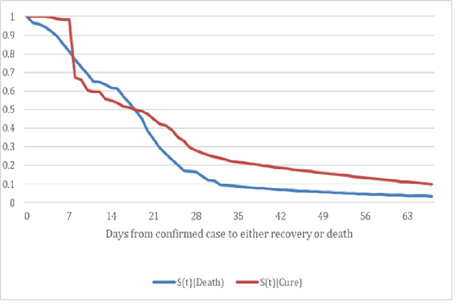
COVID-19 variants seem to have become less lethal, but survival functions estimates for successive variants have to account for deaths and recoveries from earlier variants. The same methods work for quantifying product reliability growth due to product changes, not MTBF growth as in [Duane, AMSAA Crow]. Maximize the log likelihood function or minimize the sum of squared errors between observed failure mode counts and actuarial hindcasts ∑a(s|mode)n(t-s), s=1,2,…,t, of past failure mode counts, simultaneously, as functions of the conditional distribution functions G(t|category) (likelihood) or conditional actuarial rates a(s|mode)=(G(t|mode)-G(t-1|mode))/G(t|mode).
If you would like examples of multivariate survival function or reliability function estimation, without life data, ask or send data.
References
L. A. Baxter, “Estimation from Quasi Life Tables,” Biometrika, Vol. 81, No. 3, pp. 567-577, Aug., 1994
L. H. Crow, “Methods for Assessing Reliability Growth Potential,” IEEE Proceedings Annual Reliability and Maintainability Symposium, pp. 484-489, 1984
J. T. Duane, “Learning Curve Approach To Reliability Monitoring,” IEEE Transactions on Aerospace, Vol. 2, pp. 563-566, 1964
S. G. Eick, W. A. Massey, and W. Whitt, “The Physics of the Mt/G/Infinity Queue,” Ops. Res. , vol. 41, pp. 731-742, 1993
L. L. George, “Estimate Reliability Functions Without Life Data,” ASQ Reliability Review, vol. 13, pp. 21-25, 1993
L. L. George, “A Note on Estimation of a Hidden Service Distribution of an M/G/Infinity Service System,” Random Samples, ASQC Santa Clara Valley, June 1994
L. L. George and A. Agrawal, “Estimation of a Hidden Service Distribution of an M/G/Infinity Service System,” Naval Research Logistics Quarterly, vol. 20, pp. 549-555, 1973
L. L. George, “Renewal Estimation Without Renewal Counts,” ASQ Tech Briefs, Vol. 2, 2008
U. Grenander, “On the Theory of Mortality Measurement,” Skandinavisk Aktuarietidskrift, 39, parts I and II, pp. 70-96 and 125-153, 1956
Albert W. Marshall and Frank Proschan, “Maximum Likelihood Estimation for Distributions with Monotone Failure Rate,” Annals of Math. Statist., vol. 36, pp. 69-77, 1965
Noel Mirasol, “The Output of an M/G/Infinity Queuing System is Poisson,” Operations Research, Vol. 11, No. 2, pp. 282-284, Mar.-Apr., 1963
Mike Tortorella, “Life Estimation from Pooled Discrete Renewal Counts,” published in: Jewell, N.P., et al., (eds) Lifetime Data: Models in Reliability and Survival Analysis, Springer, Boston, MA, 1995

great techniques, but its a little disingenuous to state that MDT has stopped publishing sales information for their cardiac rhythm products when someone informed Medtronic they had estimated reliability based using those figures.
Medtronic has been publishing controlled study performance data continuously for several decades. The reports (which contain sales #’s) through 2004 are readily accessible on their public website.
https://productperformance.production.argo-prd.eks.mdtcloud.io/productperformance/past-reports.html
The oldest issue available on the website is #51 from 2004. Considering a twice a year publication, the issue numbers infer this has been published since the 1980s. So please stop inferring MDT hides their cardiac device product performance and took action to prevent 3rd parties from estimating product reliability.
on behalf of Larry:
Thank you for your comments and for the link to Medtronic’s reliability reports. I read the latest, 2025 report. It does not contain the lifetime data used to make the Kaplan-Meier reliability estimates.
In Public Health Statistics class, the lecturer said “the sine qua non” of statistical publication is that the reader should be able to reproduce the results of the publication.
A few years ago, Medtronic used to advertise the annual sales and failure counts for one pacemaker, from which I made nonparametric max. likelihood reliability estimates, which agreed with Medtronic’s Kaplan-Meier estimates. Medtronic quit advertising sales and failure counts. They still don’t publish the data statistically sufficient to reproduce their results. Furthermore, their 2025 report show 95% confidence bands on reliability computed from pointwise confidence limits for each age. That misleads readers into thinking reliability will stay within the bands with 95% probability.
OK, it’s disingenuous of me to criticize Medtronic for hiding data that allowed me to verify their reliability estimate, because I want other people to estimate their products’ and parts’ reliability from sales and failure counts, available from data required by GAAP. The article gives the URL to a Google sheet to do it.
I will recommend that Fred publish your comment, but I will probably try to get Fred to allow me to make this email in reply to your comment.
Sincerely yours,
Larry George
Lifetime data is not required for nonparametric reliability estimation!
[Xmas Newsletter ca. 2012 said…] The US FDA docket, “Strengthening Our National System for Medical Device Postmarket Surveillance,” Sept. 2012, proposes to require unique identification on all implantable medical devices. This is unnecessary for reliability analysis and early warning, plus it risks privacy, requires a huge db, and is subject to human data entry errors. (Afghan refugee mortality surveys by the International Rescue Committee had so many errors: e.g. age at death after survey date!, that I had to use current status statistics: ASA Joint Statistical Meeting, San Diego, Aug. 2012) There may be other unique identification reasons besides reliability, but, if reliability problems were discovered, hospital implant records would be sufficient to notify affected patients. I submitted an official FDA comment proposing the use of installations and failure counts, which are required by GAAP and are statistically sufficient. This worked for pacemakers. The comment was met with resounding silence.
I still offer to make nonparametric estimates of reliability or survival functions, from sales and returns counts: even for multiple return modes, even for renewal processes from your data: even from revenue, service costs, and bills of materials data required by GAAP.