
Introduction
In some of my articles, I have referred to The Central Limit Theorem, a development in probability theory. It can be stated
“When independent identically distributed random variables are added, their normalized sum tends toward a normal distribution (informally a “bell curve”) even if the original variables themselves are not normally distributed.”
We can apply this principle to many practical problems to analyze the distribution of the sample mean. In this article, I provide graphical and mathematical descriptions and a practical example.
A Uniform Distribution
To illustrate the Central Limit Theorem, consider the variable x, which is uniformly distributed between a lower limit (a) and an upper limit (b), described as. Using Minitab, 1000 samples of x from the distribution is were simulated. The x values were plotted as a histogram, figure 1.
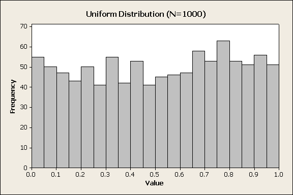
Figure 1
Since there are 20 equal sized intervals, we expect 50 samples per interval. The histogram shows the frequency in each interval is about 50 and the average is about 0.5.
Now consider the average of two x’s, i.e., $-\bar{x}=(x_2-x_1)/2-$. In this case, I used the first sample as x1 and sampled another 1000 for x2. The averages were plotted as a histogram, figure 2.
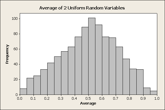
Figure 2
Now the averages don’t follow a uniform distribution but appear to follow a triangular distribution. Repeating the process, the histogram of the average of 3 uniformly distributed x’s is shown in figure 3.
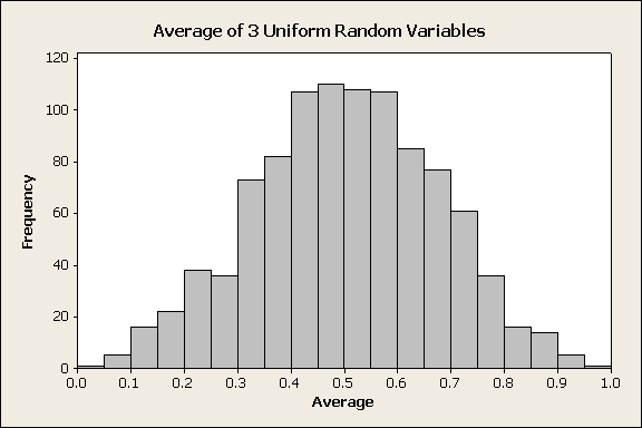
Figure 3
Now the distribution of the averages shows some curvature in the sides and some flattening of the center. Extending this process, the average of 12 uniformly distributed x’s is calculated, figure 4.
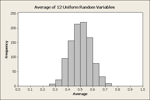
Figure 4
The distribution of the average is starting to show a bell shaped curve, i.e., a normal distribution. Note that the center remains at about 0.5 and that the variation is getting smaller.
Probability
For the uniformly distributed random variable $-x~U(0,1)-$, the average and the variance of the distribution are calculated as
$$\mu_x=\int_{0}^{1}xf(x)dx=0.5$$
where $-f(x)=1-$ for a variable distributed as U(0,1).
and
$$\sigma^2=\int_{0}^{1}(x-\mu)^2f(x)dx=1/12$$
For figures 2 to 4, 1000 samples of size n were generated for the simulation. The average $-\bar{x}-$ of each group of size n was calculated as
$$\bar{x}=\frac{1}{n}\sum_{i=1}^{i=n}x_i$$
It can be shown that the distribution average of $-\bar{x}-$ is
$$\mu_\bar{x}=\mu$$
And the variance is
$$\sigma_\bar{x}^2=\sigma^2$$
And as n get larger, the distribution approaches a normal distribution, $-N(\mu,\sigma^2/n)-$. Note that the average remains the same, but the variance decreases with increasing sample size n.
For n=12, the standard deviation of the average is
$$\sigma_\bar{x}=\sqrt{\sigma^2/n}$$
So for figure 4, the distribution of the averages of 12 samples is approximately normally distributed with an average of 0.5 and a standard deviation of 1/12. This gives a range of (0.25,0.75). This is readily apparent in figure 4 as all of the 1000 averages fall in the expected range.
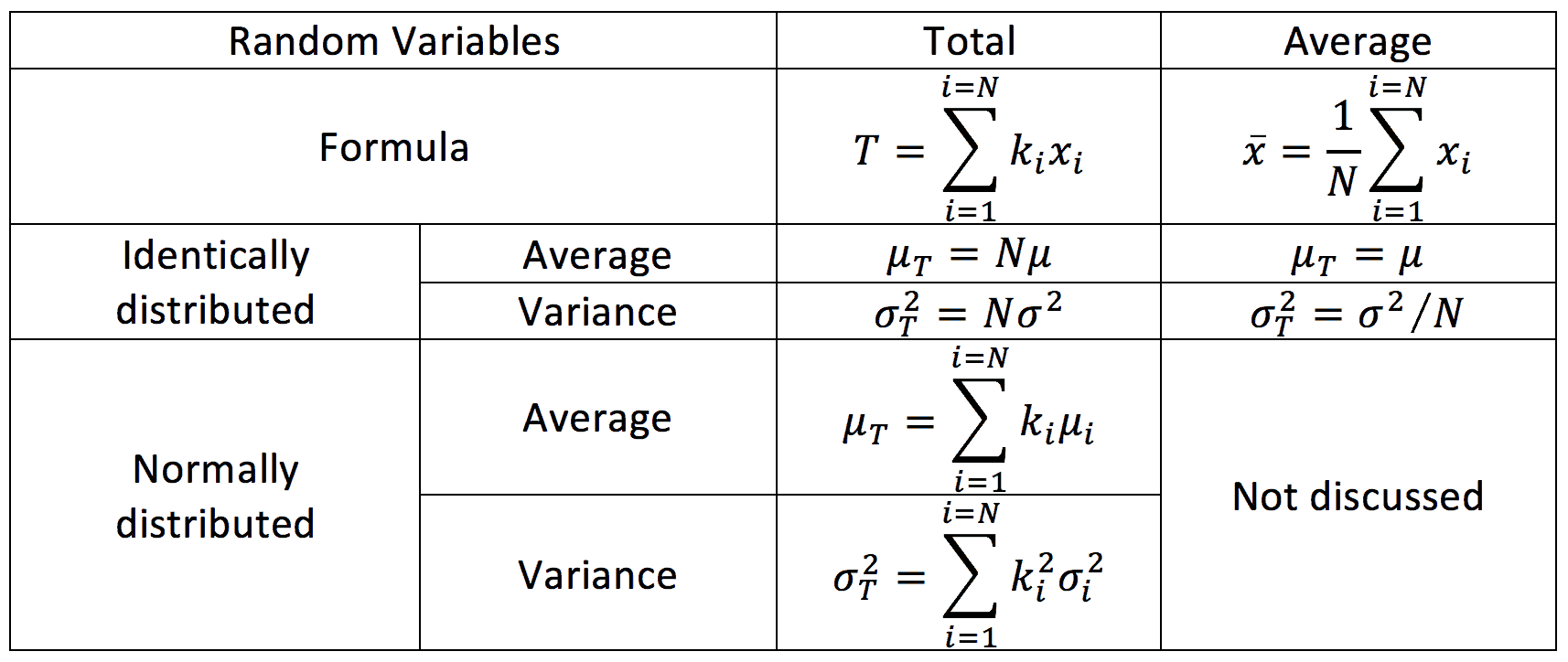
A more general expression occurs for T, a linear combinations of independent random variables x.
$$T=\sum_{i=1}^{i=n}k_ix_i$$
Here k1, k2, k3 … kn are real constants. It can be shown that the average of T is
$$\mu_T=\sum_{i=1}^{i=n}k_i\mu_i$$
This indicates that the average of a linear combination of n random variables will be the same linear combination of individual averages. Also,
$$\sigma_T^2=\sum_{i=1}^{i=n}k_i^2\sigma_i^2$$
This indicates the variance of a linear combination of n random variables will be a linear sum of the individual variances. This conclusion does not say that the T variables are normally distributed. For instance, if one of the x elements had a much larger variance than the other components, then it might control the distribution of the T variables.
The above information may be combined into a convenient table.
Example
The total power dissipated in an engine control module was being analyzed. The standard design practice was to consider a worst-case analysis. The worst-case power dissipation of the module was 34 watts. I suggested that a statistical estimate would provide a more realistic answer.
The design engineer provided the component list and the maximum power dissipated by each of the module components. Some research was required to determine the average and standard deviation of the power dissipated for each component. The average, standard deviation, and distribution type was inserted in the list to replace the fixed worst-case estimate as the information became available.
An @RISK Monte Carlo simulation provide $-\mu_T=20.75-$ watts, $-\sigma_T=0.16-$ watts, and lower and upper 3-sigma limits of (20.27, 21.23) watts, respectively. These values are considerably below the worst-case prediction.
To verify the results, the power dissipation in a module was measured as 19 watts. This was slightly less than the lower 3-sigma limit. It was a consequence that some data was not available at the time of the simulation. When the data was not available, the simulation used the worst-case component value.
The final result was that the engine control module was designed to dissipate approximately 22 watts.
Conclusions
The Central Limit Theorem describes linear combinations of identically distributed random variables. It is used to analyze assemblies or statistics that involve many elements. The information discussed above may be combined into a convenient table.
Monte Carlo Simulation provides an appropriate way to model complex systems from the distribution of component characteristics.
If you want to engage me on this or other topics, please contact me. I offer a free hour for the first contact to discuss your problem/concerns and to determine how I can help you.
I have worked in Quality, Reliability, Applied Statistics, and Data Analytics over 30 years in design engineering and manufacturing. In the university, I taught at the graduate level. I also provide Minitab seminars to corporate clients, write articles, and have presented and written papers at SAE, ISSAT, and ASQ. I want to help solve your design and manufacturing problems.
Dennis Craggs, Consultant
810-964-1529
dlcraggs@me.com
 Ask a question or send along a comment.
Please login to view and use the contact form.
Leave a Reply