
Ongoing Reliability Testing (ORT) is a way to estimate reliability function, as a function of independent variables, primarily age. This is because reliability is “the probability of successful function to specified ages under specified conditions” [O’Connor et al.].
Think of planning ORT as a design of an experiment (DoE). A DoE objective is to quantify effects of factors (independent variables) on the dependent variable, the reliability function. (The reliability and failure rate functions contain the same information, because reliability = P[Life > t] = exp[–∫a(u)du], where a(u) denotes the failure rate function and the integral runs from 0 to t.)
This article proposes answers to:
- Is ORT worthwhile?
- How many units should be on test at any time and for how long?
- How should tests be scheduled?
- What does the ORT data show?
- What should be done with units that fail ORT?
Failures often occur early at early ages, so they’re called infant mortality. Figure 1 shows microprocessor infant mortality [Intel], because the failure rate per hour in the first 50 hours is greater than subsequently, by an order of magnitude. Process defects cause infant mortality. Infant mortality may not be evident from the field failure rate, so ORT may be the only way to quantify it.

ORT is worthwhile if its value exceeds its costs by more than alternatives, if any. There may be no need for ORT, if initial tests, calibration, debugging, and burn-in extend past infant mortality. Use the data from initial tests and field reliability to estimate the early-life failure rate function. Field data may provide sufficient information for process control, and it’s population, not sample, data. However, ORT may provide estimates sooner and with a finer age scale than estimates from field data.
Compare the cost of ORT with the cost of shipping products with out-of-control process defects. If the cost of ORT is less than the cost of process defects eliminated by ORT, then ORT is worthwhile. Unlike 100% burn-in, ORT does not directly eliminate process defects. You have to use ORT information to diagnose and quantify process defects.
Design of experiments requires a model of the dependent variable as a function of independent variables. Figure 2 shows a linear approximation of a failure rate function that characterizes infant mortality. Independent variables determine the α, β, and to parameters. The linear approximation is a(t) is α+β(to–t) for t< to and a(t) = α thereafter.
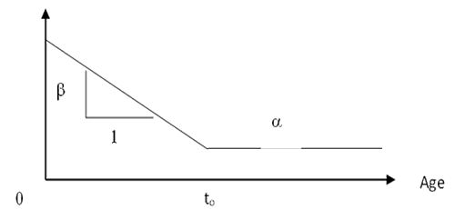
At least three test durations, t1, t2, and t3, must be used to estimate α, β, and to parameters. At least two observations must be in infant mortality segment to estimate the slope β. The most accurate estimate of the slope β is from observations at the endpoints of the slope, but, unfortunately, age zero is not a useful duration for ORT. I recommend durations to/2, to, and 2to. Guess to or use information from previous, similar products or parts. Run ORT for multiples of hours, days, weeks, or months so that human interventions are minimized. Schedule tests with a convenient greatest common divisor (GCD) such as an hour, a day, or a week.
ORT with more than one test duration is a stratified sampling experimental design. The optimum design allocates strata samples proportional to the standard deviations within strata and inversely proportional to the square roots of the cost per sample within the strata [Kish, Neyman]. The optimum stratified sample sizes satisfy
ni/n = ((Niσi)/sqrt(ci))/Σ((Niσi)/sqrt(ci)),
where ni is the stratum sample size out of a total sample of n, each stratum is assumed to have Ni members, ci = co +c1ti is the cost per unit tested, and the sum runs over all strata. Call these “Neyman proportions.” If you observe only the proportion failing, pi, then the standard deviation si is √[nipi(1–pi)] from the binomial distribution.
Because ORT replicates itself, you will obtain more short-duration samples than long-duration samples. Because shorter tests accumulate samples at greater rates, it is not necessary to test so many simultaneously.
The strata are [0,to/2], (to /2, to], and (to,t3]. For example, suppose you’re allowed at most 200 to be on test simultaneously. Compute the Neyman proportions for some arbitrary large population N with large populations Ni in each stratum.
Suppose the following estimates are reasonably close: t0 = 14 days, α= 1E–6 per day (42 FITs), β = –1E–4, and c1 = $10 per day. The probabilities for the standard deviations are computed as pi = P[Life ≤ti] = 1–exp[–∫a(u)du], where the integral of the failure rate function a(u) extends from 0 to ti. The pi values are
p1 = 0.0018, p2 = 0.00837, and p3 = 0.00839.
Table 2 shows the nearly optimum sample sizes, the actual proportions, and the Neyman proportions. This solution was obtained in a spreadsheet by changes in the sample sizes in the second column until the proportions computed in the third column agreed tolerably with the computed Neyman proportions. The number of units on test simultaneously was limited to 200 or fewer.
Table 2. Near-optimum sample sizes, proportions, and Neyman proportions
| Size | Proportion | Neyman proportion | |
| Sample 1 | 38 | 0.12752 | 0.12892 |
| Sample 2 | 145 | 0.48658 | 0.48502 |
| Sample 3 | 115 | 0.38591 | 0.38606 |
| Total on test | 197 | 1 | 1 |
| Samples per cycle | 557 | t1:t2:t3 = 1:2:4 |
This ORT plan consists of 38 units tested for one week with four repetitions, 145 units tested for two weeks with two repetitions, and 115 units tested for four weeks. Table 2 shows the expected numbers of samples to failure. These numbers should be enough to monitor production.
Table 3. Expected number of samples until failure is observed in the sample
| Duration, weeks | Expected number of samples to failure | |
| Sample 1 | 1 | 15 |
| Sample 2 | 2 | 0.82 |
| Sample 3 | 4 | 1.04 |
HOW SHOULD THE ORT DATA BE USED?
From the observed failure proportions, p1, p2, and p3, estimate the stratum failure rates:
a1 = p1, a2 = p2/(1–p1), and a3 = p3/(1–p1–p2).
Note that these failure rate estimates may be in unequal age intervals.
The sum of squared errors (SSE) for the piecewise linear model is either
[Estimated a1–α–β(to–t1)]2+[Estimated a2–α–β(to–t2)]2+[Estimated a3–alpha]2 or
[Estimated a1–α–β(to–t1)]2+[Estimated a2–α]2+[Estimated a3–alpha]2,
depending on whether t2 < to or t2 >= to. Minimizing the first SSE expression yields parameter estimators that are too ugly for publication in this article. Contact me for the formulas or a spreadsheet that computes them. Minimizing the second SSE expression yields the reasonable appearing parameter estimators:
α = (a2+a3)/2,
β = (2a1–a2–a3)/(2t1), and
to = 2t1.
Check which set of parameter values to use by checking whether t2 < estimated to or t2 >= estimated to. Use the first set if t2 < estimated to. Alternatively, use the parameter values that yield the smaller SSE value.
Compute parameter estimates from the failure rates. If the end of infant mortality to isn’t where you thought it was, revise the strata boundaries and reschedule accordingly. If the parameter estimates differ significantly from those used to select the sample sizes, again optimize sample sizes and reschedule accordingly.
STATISTICAL PROCESS CONTROL IN ORT
The direct approach is to estimate confidence limits on the age-specific failure rate function at the test times and see whether ORT estimates drift above the confidence limits. [Clark and Leon monitored three sequential tests.]
A presentation and article [Wu and Meeker] plots age-specific failure rates from production in different calendar intervals. The authors recommend monitoring the plots for changes. That has value, but warranty failures may have causes other than process defects.
Neither alternative is as convenient nor as immediate and direct as specifically monitoring infant mortality itself. The probability of an infant mortality failure is approximately equal to the triangular area toβ/2 under the sloped portion of the age-specific failure rate function in figure 2. Monitor toβ/2 with a process control chart. Every four weeks in the example, one ORT cycle will be completed, from which an estimate of toβ/2 can be computed and plotted on a control chart.
Set the upper control limit (UCL) by using the empirical standard deviation of toβ/2 under control; i.e., compute the standard deviation of toβ/2 from prior ORT cycles during which production seemed under control. Set the UCL at two or three standard deviations above the average toβ/2, depending on how fast you want to be warned of deviations and how tolerant you are of erroneous warnings (assuming toβ/2 has an approximately normal distribution).
If you don’t have any ORT data, use the failure rate function estimated from field data or use the ORT data from a comparable product to estimate toβ/2 and its standard deviation. Alternatively, approximate the standard deviation with the square root of either
(4n1p1(1–p1) + 172n2p2(1–p2) + 192n3p3(1–p3)/4]/576 or
(4n1p1(1–p1) + n2p2(1–p2) + n3p3(1–p3))/4
respectively, depending on whether the parameter estimates come from the first or the second SSE expression.
These formulas approximate the variance of toβ/2, assuming that the failure probabilities and their covariances are small. It was derived by substitution of the formulas for the estimators of to and β into Var[toβ/2] and simplification, with t1 = to /2, t3 = 2to, and Var[ai] ~ Var[pi].
Also monitor α, the constant failure rate at the bottom of the bathtub curve, if you’re interested. Use Hotelling’s T2 to monitor α and toβ/2 simultaneously. Alternatively, monitor the infant mortality triangle plus the rectangle underneath it, αto(1+β/2).
WHAT SHOULD YOU DO WITH FAILED UNITS?
If the analysis is necessary and informative, analyze failed units and record the results. Then repair the failed units and put them back on test for a long time, or ship them. Track them by serial number so that you can efficiently compare the reliability of repaired and new units, to quantify the efficacy of repairs. MIL-STD-2155, FRACAS, and MIL-STD-1520B comment on disposition of failed units. They recommend tracking of reworked units so that their field reliability can be estimated. They also recommend root cause analysis
PROTOTYPE DORT PLAN
Sampling Plan Objective: The number of units per ORT cycle shall be sufficient to detect a change in infant mortality of a specified percent within a specified time, limited by facilities and cost.
Test Conditions:
- Normal or accelerated as appropriate.
- Cycle on and off if that reveals infant mortality.
Duration and Sample Sizes:
- Choose test times to span infant mortality, with one in the middle of infant mortality, one as near to the end as possible, and one afterward in the supposedly constant failure rate portion of product life.
- Schedule them with as large a GCD as convenient: hour, day, week, or month.
- Choose sample sizes as large as possible in approximately the Neyman proportions.
Procedure:
- Set up and test randomly chosen units. Record the start times.
- Run samples for specified times. If possible, monitor for failures and record failure times. If not possible, record failure counts.
- Repeat when shorter test durations are over and when the ORT cycle is complete.
- Data Collection and Analysis
- Record failure time or counts and failure modes for units that fail. Record test times for those that don’t fail.
At the end of each ORT cycle, compute the parameter estimates. Is tonear where it was expected to be? If not, revise test durations. Do parameter estimates approximate previous or assumed values? If not, revise sample sizes.
Compute toβ/2, and plot it on the SPC chart. Blow the whistle if it exceeds the UCL; otherwise, revise the UCL on toβ/2 occasionally.
CORRECTIVE ACTIONS?
Deal with failed units according to MIL-STD-1520B. Do failure analysis on failed units if appropriate and necessary. Repair and ship if appropriate.
If the cycle estimate of toβ/2 > UCL, do failure analysis and root cause study of failed units tested since the last increase in toβ/2. Compare with failure analyses of earlier failures.
Initiate suitable process corrective action, depending on the root cause, if the expected cost of failure exceeds the expected cost of the fix. Change design only if necessary to prevent process defects.
ORT could be political. Physical constraints limit how many products can be tested simultaneously. Companies may need to ship all available products at the end of a quarter. Make sure your ORT plan incorporates such constraints.
Note: this article originated from ASQ Reliability Review, Vol. 22, No. 4, pp. 5-13, Dec. 2002.
REFERENCES
Clark, W. David and Ramón V. León, “Detecting Changes in Field Reliability Using Data from a Complex Factory Screen,” Joint Statistical Meeting 1998, Dallas, Texas, August 11, 1998
George, L. L. and Yat-H. Lo, “An Opportunistic Look-Ahead Replacement Policy,” Annals of SOLE, Vol. 14, No. 4, Winter 1980
Intel, Figure 1 is based on http://www.intel.com/support/fittable.htm, now gone. Similar data was available from http://www.intel.com/support/controller/mcs96/components/fittable.htm, also gone.
Kish, L., Survey Sampling, page 93, John Wiley and Sons, New York, 1965
MIL-STD-1520B, “Corrective Action and Disposition System for Nonconforming Material,” DOD, Washington, DC, 3 July 1980
MIL-STD-2155(AS), “Failure Reporting, Analysis, and Corrective Action System,” AMSC N3637, DoD, Washington, DC, 24 July 1985
Neyman, J., “On the Two Different Aspects of the Representative Method: the Method of Stratified Sampling and the Method of Purposive Selection,” Journal of the Royal Statistical Society, vol. 97, pp. 558-606, 1934
O’Connor, Patrick D. T., David Newton, and Richard Bromley, Practical Reliability Engineering, third edition, New York: John Wiley & Sons, 1996
Wu, H. and W. Q. Meeker, “Early Detection of Reliability Problems Using Information from Warranty Databases,” Trondheim, June 2002. An article with the same title appears in Technometrics, vol. 44, no. 2, pp. 120-133, May 2002

Leave a Reply