Estimate Reliability Functions Without Life Data

ASQC Reliability Review, Vol. 13, March 1993

This paper shows how to estimate field reliability functions from ships and returns. It offers to estimate field reliability functions from your data. It suggests how you can use these estimates to improve service and inventory management. [Links to Google Sheet and user guide follow the paper.]

You can estimate field reliability functions without life data. You don’t need to know each part’s time to failure. In fact, if you don’t know times to failures, you have to estimate field reliability functions from ships and returns, unless you have a sample of times to failures, and some of the sample failed.

Ships tell how many products were shipped, and returns tell how many parts were returned or replaced, periodically. From ships and returns, you can estimate population field reliability functions, not sample functions. This is because ships and returns contain sufficient information to estimate field reliability functions.

These estimates will revolutionize service and inventory management. Forecasting and service inventory methods once possible only for carefully tracked products like aircraft engines can now be applied to any repairable products:

Designers will verify inherent reliability and control early wearout
Manufacturers will plan burn-in and control infant mortality
Service managers will forecast requirements and set stock levels.

These estimates reveal an unrecognized segment of the bathtub curve caused by retirement or incursion of other suppliers. Recognizing retirement helps reduce spare parts inventories as products become obsolete.

FIELD RELIABILITY FUNCTIONS AND THEIR USES

“Reliability is the (prob)ability a product does its required function for a specified amount of time.” I added “(prob)” because I use probability to quantify reliability. Here are three service management alternatives.

Reality: If you don’t know reliability functions, service management is management of uncertainty. You don’t know when parts will fail. You don’t even know failure times of parts when they fail, even if failed parts are returned, because you don’t know which products they came from. It’s too costly to track each product and its failures and too costly to track a sample. Life is uncertain, but why should work be uncertain too?

Ideal: If service managers knew all times to failures, service management would be routine. You would:

Recognize infant mortality caused by process defects
Know how long to burn in
Obtain early warning of defects or higher-than-predicted failure rates
Verify inherent reliability or recalibrate reliability predictions
Recognize design defects caused by premature wearout
Verify fixes and observe the fraction of customers adopting them
Forecast repair workload and spares requirements
Stock spare parts when needed
Know warranty costs and set warranty reserves accurately
Recognize product retirement and avoid obsolete spares

Unfortunately, there’s no way to know failure times, until they occur, and even then it’s difficult to get failure time data.

Possible: If you knew field reliability functions, service management would be management of randomness. You wouldn’t know exactly when parts would fail, but you would know their reliability functions. You would:

Recognize infant mortality by testing for decreasing failure rate functions
Set burn in time so expected infant mortality cost equals burn in cost
Test whether actual return rates differ significantly from expected return rates
Test whether the failure rate differs significantly from its prediction
Test for a prematurely increasing failure rate function
Test whether the reliability function after a fix differs significantly from before
Forecast expected returns and their distribution functions
Use the forecasts to set stock levels and reorder points
Estimate warranty costs as fraction failing within warranty, and set reserves to have sufficiently high confidence
Recognize onset of retirement and reduce spare parts inventory accordingly

Fortunately there is a way to estimate reliability functions even if you don’t know service times to failures. Wouldn’t you rather manage randomness than uncertainty?

REVOLUTIONIZE FORECAST OF SERVICE REQUIREMENTS

Before estimation of field reliability functions from ships and returns, service managers forecast workload and spares requirements two ways:

Consumer and repairable products—extrapolate previous sales [of spares, or warranty returns]
High-cost repairable equipment—use installed base, operating hours, goes-into theory and failure rate function to estimate requirements

After estimation of field reliability functions from ships and returns, service managers of repairable systems can forecast workload and spares requirements just like people who manage high-cost repairable equipment:

Throwaway consumer products—no change
High-cost repairable equipment—no change
Repairable products—use ages of installed base, goes-into theory and failure rate function to estimate requirements

Forecasting repairable parts requirements will change service management from management of uncertainty to management of randomness. The forecast of requirements will be done by the actuarial method [AFM 66-1] instead of by extrapolating past returns. Goes-into theory computes the numbers of parts shipped given product ships and bills of materials.

NOTATION

The (discrete) reliability function is R(t) = P[Life > t] = 1-∑p(s), s=0,1,…,t, where s and t stand for calendar time units like months. The discrete probability density function p(s) is P[Life=s]. The discrete failure rate function is p(s)/R(s), also known as the actuarial failure rate function. Ships are denoted by n(t) and returns are by r(t). Although time units appear the same in p(t), n(t) and r(t), they represent different times. Time in p(t) represents age, calendar time since shipment of a unit of a product. Time t in n(t) and r(t) represents calendar time since product introduction, or the time since shipment of unit number one [or the time since shipment of a cohort].

FIELD FAILURE RATE FUNCTION DIAGNOSES DEFECTS

The bathtub curve in figure one helps diagnose defects. Process defects in manufacturing, delivery or installation cause infant mortality. Design defects cause premature wearout. Coincidence or absence of infant mortality and wearout cause a constant failure rate. The theorem from when hell freezes over [Barlow and Proschan], pages 18-21) says if a system has enough parts, all independent, in series, with no predominant failure rates, replaced immediately on failure, and if they have failed enough times, then system failure rate is constant, after a long time. Most repairable systems don’t get used that long.

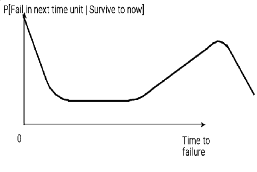
Figure 1. The bathtub curve failure rate function

Figure one also shows a line segment you’ll see if you wait long enough. The tail of the wearout failure rate segment is caused by retirement, attrition, or incursion of other vendors. You need to estimate that segment to liquidate spare parts inventories before they become obsolete.

WOULDN’T YOU PREFER POPULATION STATISTICS?

“People respond to the ratio of sample size to population size not to the absolute sample size.” [Tversky and Kahneman, paraphrased].

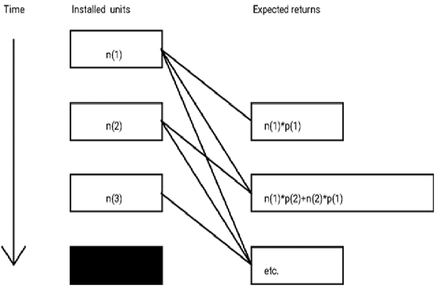
Even though actual failure times are unknown, ships and returns are sufficient to estimate the distribution of time to failure, 1-R(t). Figure 2 shows that the unknown distribution represented by the p(t) values can be estimated from known ships and returns, n(t) and r(t). In that figure, the only unknowns are the p(t). They can be estimated by several methods. Furthermore, such estimates are population estimates because they use all ships and returns, not a sample. Such estimates may be sufficient statistics.

Statistically, sufficient means the conditional distribution of ships and returns data, given the reliability function estimator, is independent of the unknown reliability function. In other words, the reliability function estimator contains all information in the ships and returns data relevant to the reliability function.

Using ships and returns actually yields an estimate of the distribution of life time plus sell-through time. If sell-through time is significant, compute the field reliability function by convolution of total time minus sell-through time. Sell-through and life times are independent.

MLE and LSE Estimate of Reliability Functions

MLE (Maximum Likelihood Estimation) maximizes the probability of observed ships and returns as a function of the unknown reliability function. Reference by [George and Aggrawal] gives the MLE. Maximum likelihood estimates are generally sufficient statistics.

Before using the MLE, test whether ships are a stationary Poisson Process (constant shipping rate). The test in [Cox and Lewis], tests whether a regression line fitted to cumulative ships is a linear function of time, equivalent to a constant shipping rate. Then test whether mean equals variance, because a Poisson Process has equal mean and variance.

If shipping rate is not a stationary Poisson Process, use LSE (Least Squares Estimation). Minimize the sum of squared differences between expected and actual returns as a function of the unknown discrete probability density function p(t).

COMPUTATIONS

Suppose you introduced a product one month ago. You know ships, the first month sales, n(1). You know returns, those parts returned or failed in the first month, r(1). What’s the estimate of p(1)? Right, r(1)/n(1). That’s the least squares estimate too. Here’s the proof.

The sum of squares to be minimized is [Expected returns – actual returns]= [p(1)*n(1)-r(1)]. Take the derivative with respect to p(1) and set it to zero; 2*n(1)*[p(1)*n(1)-r(1)] = 0.

Solve for p(1) and get r(1)/n(1). Equations become more complicated as ships and returns accumulate, but the LSE remains the same; minimize the squared difference between expected and actual returns with respect to p(.)

Minimize ∑{∑[p(t-s+1)*n(s))]-r(t)]²} where the outer sum is over t=1,2,… and the inner SUM is over s=1,2,..,t. Minimization is over values of p(.). ∑[p(t-s+1)*n(s))] is an actuarial forecast of returns.

The upper limit on the outer sum [on time t] is the number of months the part has been in the field. (You can’t estimate field reliability for ages greater than the age of the oldest product, unless you make assumptions about future field reliability.)

Figure 2. Ships, returns and failure probabilities

Formulas for expected returns in the LSE equation depend on disposition of returned parts and the effects of repairs:

Failed products are taken out of service
Returned parts are destroyed
Replacements counted in ships
Recycled returns are good-as-new, good-as-old, or hysterecal
Combinations and converses of these.

Mathematica™ Minimizes the LSE Equation

Mathematica solves the unconstrained LSE equation symbolically, for a few months’ data. I copy the symbolic formulas into spreadsheets for estimation for many products. Figure 3 shows the formulas for a two-period old product. You won’t like the solutions for three, four and five period old products, and Mathematica won’t solve any larger problems symbolically. If your ships and returns data is annual, you probably have five or fewer years of data.

The p(t) probability values that minimize the unconstrained LSE equation may be negative! A probability distribution must be nonnegative and add to 1.0. To get nonnegative p(t) values, transform the p(t) when you use Mathematica. If probabilities are small, the probability of violating the 1.0 constraint is negligible.

Mathematica gives numerical solutions for problems with more than five periods, but it frequently gets trapped in local minima. Execution time is interminable, so use other methods.

Simplex Nonlinear Optimization Code Resource

To speed up minimization, I implemented the simplex nonlinear optimization from [Cox and Lewis] as an Excel code resource. I put it in a loop to handle multiple products. It too gets trapped in local minima, but quickly. Then I restart optimization from different initial values.

Solver Minimizes the LSE Equation Subject to Constraints

Excel’s Solver also does constrained, nonlinear optimization using the Levenberg-Marquardt method, [Press et al.], so constrain the p(t) to be nonnegative. To avoid getting trapped in local minima, Solver anneals. That is, if little improvement occurs after several successive iterations, Solver tries new starting points.

(* This Mathematica notebook solves for the actuarial failure rate function using Least Squares Estimation, for 2 periods. *)
Array[n,2];
Array[r,2];
Array[p,2];
e[1]=p[1]*n[1]
e[t_]:=Sum[n[s]*p[t-s+1],{s,1,2}]
LS[n_]:=Sum[(r[t]-e[t])^2,{t,1,n}]
Solve[{D[LS[2],p[1]]==0,D[LS[2],p[2]]==0},{p[1],p[2]}]
            n[2]*r[2]    -(n[1]*r[1]) - n[2]*r[2]
{{p[1] -> -(---------) - ------------------------, 
              n[1]2                n[1]2
             (-n[1]2  - n[2]2 )*r[2]
   p[2] -> -(---------------------) + 
                     n[1]3
     n[2]*(-(n[1]*r[1]) - n[2]*r[2])
     -------------------------------}}
                  n[1]3

Figure 3. Mathematica solves for p(1) and p(2) analytically. D denotes derivative, := denotes definition, == denotes comparison, and -denotes equals.

HARD DISK DRIVES

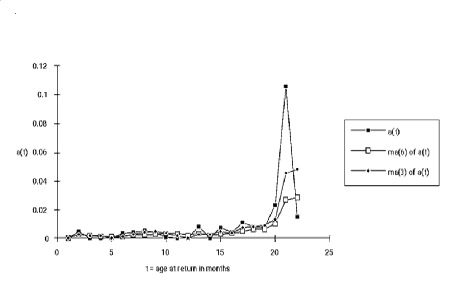
Figure 4 shows the failure rate function estimate, a three-month moving average, and a six month moving average, for a widely used hard disk drive. Premature wearout occurs at 20 months, or else the first few month’s ships were defective. Remember, this estimate is for a product fielded for 22 months, so only the oldest ships contribute to the estimates of p(20), p(21) and p(22). I segregated returns by ship date and tested the hypothesis that the reliability function that the first three months’ ships was worse than that of later ships. I accepted the hypothesis.

Figure 4. Failure rate function for a hard disk drive [ma(j) stands for moving average of lag j]

FREE OFFER AND RECOMMENDATIONS!

Send your data: ships, returns and goes-into data. Tell which parts go into which products and how many go in each product. Tell the dispositions of failed products, returned parts and repairs. Are failed products repaired? If so, is the failed part replaced or repaired? Do replacements or repairs make part good as new, good as old, or somewhere in between? Are spares and replacements counted in ships? Send DOS or Macintosh, spreadsheet, dBASE or text format. Send by modem or fax, CompuServe or MCI Mail if you’re in a hurry. [That was in 1993. Email pstlarry@yahoo.com in 2025.]

I’ll return nonparametric, discrete reliability and failure rate function estimates. I’ll sometimes use a kernel estimator to extrapolate and smooth the failure rate function. I’ll fit your reliability function if I can. Weibull fits PC board and disk drive infant mortality very well.

You can no longer complain that you don’t have life data. That’s no excuse for not knowing your products’ and its parts’ reliability functions. If you have returns data, spare parts sales data or any record related to monthly parts demands, you can estimate reliability functions. I’ll get you started. Do it now, before anyone realizes you’re not using your data to improve product reliability and service existing products.

REFERENCES

Air Force Manual 66-1, “Maintenance Management,” Washington: Department of the Air Force, August 1972

Barlow, R. E. and F. Proschan, Mathematical Theory of Reliability, Wiley, New York, 1965

Tversky, A. and D. Kahneman, “Judgement under Uncertainty: Hueristics and Biases,” Science, Vol. 185, pp. 1124-1131, 1974

George, L. L. and A. Aggrawal, “Estimation of a Hidden Service Distribution of an M/G/∞ Service System,” Naval Research Logistics Quarterly, Vol. 20, No. 3, pp. 549-555, 1973

Cox, D. R. and P. A. W. Lewis, The Statistical Analysis of a Series of Events, Methuen, London, 1966

Press, W. H. et al, Numerical Recipes, Cambridge University Press, New York, 1986

RELIABILITY ESTIMATION SPREADSHEET CIRCA 1981

This is a link to a public Google Sheet of the nonparametric maximum likelihood estimator from ships and returns counts.

https://docs.google.com/spreadsheets/d/1fb_pjwygp_2CUeayNEV4PAX6wyR8sdWqPr76qeJ_n4I/edit?gid=0#gid=0

This article explains how the Google sheet works.

L. L. George, “How Can You Estimate Reliability Without Life Data?” Weekly Update, https://accendoreliability.com/can-estimate-reliability-without-life-data/#more-416328, May 2022.

Goes-into or “gozinto” theory is explained in https://accendoreliability.com/gozinto-theory-parts-installed-base/#more-417514/