Kaplan-Meier Reliability: What Could Possibly Go Wrong?

SAS, JMP, R-”Survival”, Minitab, ReliaSoft, XLStat, and perhaps other statistics programs offer the Kaplan-Meier nonparametric reliability estimator as a default. Take credit for using nonparametric reliability estimation and avoiding unwarranted assumptions. What could go wrong using the Kaplan-Meier estimator?

• Cohorts could be non-stationary, random processes! 
• Failures could be recurrent process counts, not dead-forever! 
• Lifetime data depends on the censoring process(es); e.g., competing risks!
• Greenwood’s variance estimator errs! Covariances are missing!
• Alternative estimators could be more efficient than Kaplan-Meier!

Are you using all the information in data available from population data required by GAAP? If you don’t have lifetime data, use periodic failure counts. This article describes an example where the Kaplan-Meier estimator from grouped lifetime data is less efficient than using periodic failure counts, even though you don’t know which cohort they came from! 

Data Alternatives

Which would you prefer: censored lifetime failure counts grouped by period cohorts in Nevada table 1, or periodic cohorts and failure counts in table 2, without knowing which cohort failures came from? 

Table 1 “Nevada Charts to Gather Data,” by Fred Schenkelberg. Failure counts by cohort are in the body of the table https://accendoreliability.com/nevada-charts-gather-data/.

Month	Ship	Jan	Feb	Mar	Apr	May	Jun
Jan	3519	3	6	3	7	10	3
Feb	6292		3	8	20	35	24
Mar	7132			8	13	25	31
Apr	5633				4	13	6
May	4222					5	8
Jun	4476						6
Sums		3	9	19	44	88	78

Table 2 Periodic cohort ships and failure counts, sums of monthly failure counts from bottom row of table 1.

Period	Ships	Failures
Jan	3519	3
Feb	6292	9
Mar	7132	19
Apr	5633	44
May	4222	88
Jun	4476	78

In 1999 I wrote, “Tracking auto parts by serial number requires a mainframe; but tracking ships and returns requires a PC. There were ~4000 parts per ~6M Fords under warranty. With 8 bytes per part number, at least 17 bytes per VIN (typically ~55 bytes), and two bytes for age, that’s 600 Gb. (Not all that storage is needed until failure.) Ships and returns counts require a byte for vehicle ships, a byte per part for returns each month, plus bills-of-materials. That’s less than 1 Mb.”

Table 2 cohorts and period failure counts are statistically sufficient to make nonparametric reliability estimates. They are population data, available for free, from revenue and service cost data required by GAAP. Divide period unit-revenue = Σ(price/unit)*cohorts by price(s) to get cohorts.  Monthly failure counts could be derived from sums of service costs and spares sales. Use Gozinto theory and BoMs to convert product cohorts into parts’ cohorts by age. Use maximum likelihood or least squares to derive reliability estimator alternatives to Kaplan-Meier.

Rants about the Kaplan-Meier Estimator

If lifetime data is periodic, grouped failure counts by ship period or cohort, such as in Nevada table 1, then people may use the Kaplan-Meier nonparametric reliability estimator. That estimator assumes that censoring is non-informative, i.e., that censoring doesn’t depend on survival times, and that censored survivors would have same life distributions as failed units (with longer lifetimes). Statistical software doesn’t check conditions for Kaplan-Meier validity; SAS knows the competing risk estimator is not Kaplan-Meier. [George Dec. 2024, Liu et al.]

Greenwood’s formula underestimates the variance of Kaplan-Meier reliability function estimates. Greenwood’s formula is asymptotic and requires an unbiased reliability estimator. Covariances of reliability estimates at different ages are neglected: COV(R(s), R(t)) in confidence bands and forecasts? Others have observed other limitations on the Kaplan-Meier estimator:

• Rupert G. Miller Jr., “What Price Kaplan-Meier?” Describes the cost of nonparametric estimate vs. a parametric survival function: Akaike Information Criterion with k parameters, AIC = 2*k-2*lnL(nonparametric(k)) vs. AIC = 4 or 6-2*lnL(parametric(2 or 3)), where lnL is log-likelihood function, (k=periods for nonparametric distributions.) and 2 or 3 is the usual number of parameters for parametric distributions.
• Meier, Paul, et al. “The Price of Kaplan-Meier,” is a rebuttal of Miller’s article: the more parameters you use the better parametric distribution fits. Maybe not according to Akaike Information Criterion.
• Piovani et al., “Pitfalls and perils of survival analysis under incorrect assumptions:…” describes the joint dependence and COVID-19 deaths and censored survivors (competing risks). 
• Tomas Bencomo, “Kaplan-Meier Mistakes,” says multivariate methods,…, should be used! [For example, joint distribution of time from case to recovery or death.]
• Dependence among competing risks invalidates the Kaplan-Meier estimator [Walton].

What’s new? Reviewed? Re-ranted?

The nonparametric maximum likelihood reliability estimator (npmle) from Fred’s periodic ships and failures (table 2) beats Kaplan-Meier!!! The npmle from multiple cohorts is not Kaplan-Meier for each cohort! Cox’ proportional hazards model also beats Kaplan-Meier for periodic cohorts. Cohort covariance estimates provide confidence bands on reliability function estimates and variance of actuarial forecast.

The Kaplan-Meier estimator may be invalid due to ignoring cohort nonstationary, variability, or competing risks. Confidence bands on reliability functions may be invalid, and variance of forecasts could be wrong, due to ignoring covariances. Confidence bands could be pointwise confidence limits, for one age only, computed from normal distribution with Greenwood’s variance estimator. Covariances are needed for confidence bands [Hall-Wellner] and for the variance of actuarial forecasts [George, Dec. 2024]. 

Solutions: Incorporate cohort variability in maximum likelihood or least squares estimation. Use nonparametric maximum likelihood reliability estimates, multivariate if there are competing risks; e.g., COVID-19 recovery or death. Compute variance-covariance matrix of estimates and use it in forecast variance and confidence bands. 

Alternative Nonparametric Likelihood Functions

Use maximum likelihood if you want a single reliability estimate, assuming cohorts are independent and identically distributed. For Nevada-table grouped (by cohort) failure counts, the likelihood function could be Π(Poisson(λ(t)]*Binomial[d(t), n(t), a(t)]), t=1,2,… where λ(t) is cohort size rate, d(t) are deaths, n(t) are survivors, and a(t) are the actuarial failure rates conditional on survival. Use Cox’ proportional hazards model to include cohort number or season [Walton].

The Kaplan-Meier likelihood is sometimes written as ∏(1-a(t))^n(t), where a(t) is the actuarial failure rate function and n(t) is number of survivors to ages t=1,2,… The Kaplan-Meier likelihood from a Nevada table is ∏Binomial[d(t), n(t), a(t)]. The binomial combinatorial term drops out of maximization.

With random cohorts, Nevada table 1 likelihood could be ∏Poisson[λ]*Binomial[d(t), n(t), a(t)] or ∏Poisson[λ(t)]*Binomial[d(t),n(t),a(t)], where λ(t) is cohort rate, perhaps time dependent. Poisson(λ) means that cohort rate lambda equals average cohort size. Nonstationary Poisson(λ(t)) is hard to disprove [Nelson and Leemis] and yields greater likelihood. 

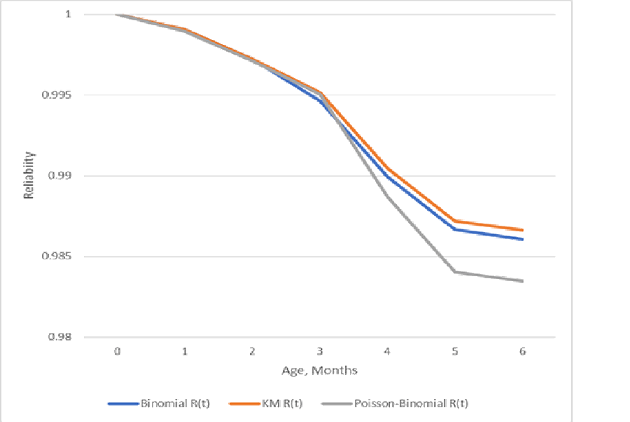
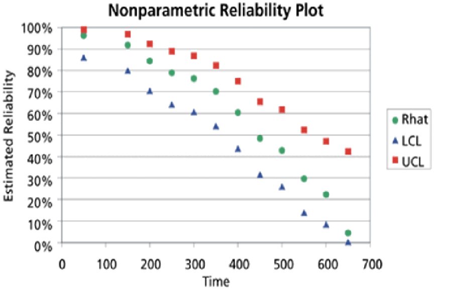
The nonparametric Kaplan-Meier likelihood from Fred’s data by cohort j maximizes L=∏Binomial[d(t; j),n(t; j),a(t)]; t=1,2,…,6, and j=Jan,…,June. Use Excel solver to maximize lnL as function of a(t) the actuarial failure rate function. The result is lnL=-55.97 and AIC = 123.95. (AIC=Akaike Information Criteria, 2k-2lnL. Small AIC is better.) The Kaplan-Meier L=∏(1-a(t))^{n(t; j)} result is lnL=-246.25, AIC = 504.5. See table 3 for comparisons of all estimators. Disagreement measures between the two Kaplan-Meier estimates are SSE = 0.000001 and Kullback-Leibler divergence = 0.000564 bits. Eyeball difference is pretty negligible (figure 2).

With stationary Poisson cohorts, the likelihood function is ∏Poisson[λ]*Binomial[d(t;j),n(t;j),p(t)] with constant cohort rate λ. The maximum likelihood λ = average cohort size 5212, lnL=-950, and AIC=1927. With nonstationary Poisson cohorts, the likelihood function is ∏∏Poisson[λ(t)]*Binomial[d(t;j),n(t;j),p(t)] with variable cohort rate λ(t), the results are better: lnL=-128 and AIC=267.

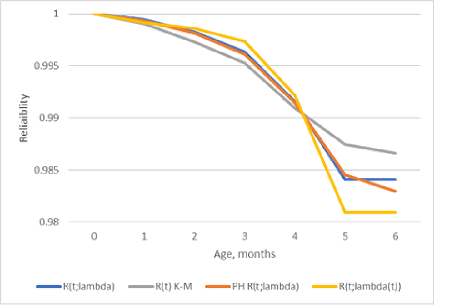
Why not estimate reliability etc. from period cohort sizes and period sums of failure counts, without lifetime data (table 2)? The likelihood function L is ∏(Poisson[s(t),λ]*Poisson[r(t),λ*G(t)]) or ∏(Poisson[s(t),λ(t)]*Poisson[r(t),λ(t)*G(t)] where s(t) are cohort sizes (“Ships”), r(t) are “Returns”, sums of failures in period t (table 2), and G(t) is cumulative probability distribution function of time to failure. This assumes the M(t)/G/infinity model of self-service queuing system with independent Poisson inputs and Poisson outputs [George 1973, Mirasol; Eick, Massey, and Whitt]. For Fred’s data, table 2, lnL=-950.6, AIC=2*13-2*lnL=1927 and λ=5212, the average cohort size. For nonstationary Poisson input process, for Fred’s data, lnL=-46.75, AIC=117.5. Nonstationary fits better according to lnL with smaller AIC than Kaplan-Meier (lnL=55.97, AIC=123.95)! The nonstationary model shows less reliability at ages 5-6 months (figure 3). 

Cox’ PH model with regression on month 1,2,…,6 almost matches the reliability estimate from ships and returns counts M/G/Infinity model. Cox’ Proportional Hazard models cohort time dependence R(age t; month x)=Exp[-∑(ao(s)*Exp[b*x])], s=1,2,…,6, x=Jan, numeric Feb,…,June, ao(s) is underlying failure rate function, and b is a regression coefficient.

According to AIC, the best, most efficient estimate from Fred’s data comes from the M(t)/G/infinity model! Wait, you might exclaim; aren’t you estimating 12 parameters, including the Poisson rates at each age t? Nope. They aren’t estimates; six of them are the observed cohort sizes!

Table 3 Summary of alternative estimators’ log-likelihood and Akaike Information Criterion

Model	lnL	Parameters	AIC
Kaplan-Meier	-56	6	124
Kaplan-Meier Poisson[λ(t)]	-128	6	267
M/G/Infinity Poisson[λ]	-950	7	1927
M(t)/G/Infinity Poisson[λ(t)]	-46.75	6	117.5
Cox PH Poisson[λ(t)]	-53.1	6	132

Variance-Covariance Matrix 

Why not estimate reliability and failure rate functions R(t; j) and a(t; j) for each cohort j in table 1? That relieves the assumption of equal censoring, because all members in each cohort get censored the same! That produces multiple cohort reliability function estimates that quantify variance-covariance matrix due to cohort variability. An actuarial forecast ∑a(s)n(t-s), s=1,2,…,t has variance ∑Var[a(s)]n²(t-s)]+∑∑Covar[a(t-s, a(s)]*n(s)*n(t-s), s=1,2,….t, where a(s) is estimate of actuarial failure rate function and n(t-s) is installed base of age t-s.

Table 4. Reliability function estimates’ variance-covariance matrix vs. Greenwood’s Kaplan–Meier variance. Cohort variances from Fred’s data are more than the K-M variances.

Age	1	2	3	4	5	Variance	K-M Var
1	1.06E-07					1.06E-07	2.96E-08
2	6.59E-08	2.25E-07				2.25E-07	9.62E-08
3	1.87E-08	-1.33E-07	4.05E-07			4.05E-07	1.71E-07
4	1.97E-08	-2.37E-07	1.24E-07	6.39E-07		6.39E-07	4.25E-07
5	-2.58E-07	-8.45E-07	2.86E-07	8.16E-07	3.78E-06	3.78E-06	7.75E-07
6	-3.84E-08	-4.05E-07	2.05E-07	-7.96E-08	-9.33E-08	1.03E-06	1.01E-06

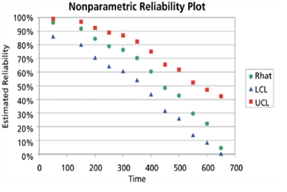
Pointwise confidence limits (figure 4) on reliability estimates R(t) are approximately R(t)±Z(a/2), because the estimates are approximately normally distributed N[R(t), ∑(t)], where ∑(t) is the variance covariance matrix of reliability estimates. These pointwise confidence limits are not confidence bands on the entire reliability function estimates a la Hall and Wellner (figure 5). ReliaSoft says these are pointwise confidence limits (R(t)±Z(a/2σ(R(t)))?), but they are asymmetric! [https://help.reliasoft.com/reference/life_data_analysis/lda/non-parametric_life_data_analysis.html/] They could be derived from limits on a(t)±Z(a/2)σ(a(t)).

Notice that confidence bands end at the oldest failure! The Kaplan-Meier reliability estimator does not extend beyond the oldest failure. What to do? Extrapolate a(t) failure rate function estimate by regression and use standard error of extrapolation to construct confidence limits or bands for ages t beyond oldest failure: R(t)=Exp[-∑a(s)], s=1,2,…,t(oldest),t(oldest+1), etc.

Figure 5 shows legitimate confidence bands [Hall and Wellner]. Notice how they expand as age increases due to fewer and fewer failures? Bands widen as t increases, because there are fewer failures at older ages.

Conclusions? Random Cohorts? Covariances?

The Kaplan-Meier reliability estimator is for censored lifetime data or for grouped-by-cohort failure time data, assuming failures are independent of the censoring processes. Do not use the Kaplan-Meier reliability estimator for renewal process failures or for competing risk data failure data. Do not use the Kaplan-Meier estimator if cohorts are nonstationary and random!

ReliaSoft, Minitab, et al. avoid cohort randomness by requiring lifetimes one-by-one along with censoring indicators. That forces cohorts of size 1. If you have grouped failure counts by cohorts (Nevada table), test for random or nonstationary cohorts (Poisson?). Compute Kaplan-Meier estimates for each cohort and use maximum likelihood for all cohorts. 

For Fred’s data, the nonparametric maximum likelihood estimator (npmle) from ships and returns with nonstationary Poisson cohorts beats binomial Kaplan-Meier estimate in statistical efficiency, goodness-of-fit, and AIC. It also shows bias in the Kaplan-Meier estimate. One example does not make a rule, but it should encourage you to check the npmle from ships and returns. How much does lifetime data cost? Does lifetime data cost more than data required by GAAP? Some work is required to extract ships and returns from population data required by GAAP. 

Have you considered sample(s) of lifetimes? Sample vs. population maximum likelihood using cohort sizes and periodic failure counts (ships and returns, cases and deaths,…) has already been analyzed [Walton].

Use population ships and returns counts to estimate reliability and failure rate functions, for all products and their service parts. Your estimates may be more statistically efficient than Kaplan-Meier estimates, AND you don’t have to collect and store lifetime data! Want reliability function estimates’ variance-covariance matrix by Cramer-Rao, Poisson bootstrap, or cohort variance-covariance? Send your data to patlarry@yahoo.com.

References

Tomas Bencomo, “Kaplan-Meier Mistakes,” https://medium.com/data-science/kaplan-meier-mistakes-48cd9e168b09/ Oct. 2019

S. G. Eick, W. A. Massey and W. Whitt, “The Physics of the M(t)/G/Infinity Queue,” Ops. Res. , 41, pp. 731-742, 1993

W. A. Hall and Jon Wellner, “Confidence Bands on Survival Functions,” Biometrica, Vol. 67, No. 1, pp. 133-143, April 1980

Kaplan, E. L. and Paul Meier, “Non–Parametric Estimation From Incomplete Data”. Jour. Amer. Statist. Assn., Vol. 53, pp. 457–481, 1958

Guixian Lin, Ying So, and Gordon Johnston, “Analyzing Survival Data with Competing Risks Using SAS® Software,” SAS Global Forum, 2012

Meier, Paul, et al. “The Price of Kaplan-Meier.” Jour. Amer. Statist. Assn, Vol. 99, No. 467, pp. 890–896, https://www.jstor.org/stable/27590457/, 2004

Rupert G. Miller, Jr. “What Price Kaplan-Meier,” Biometrics, Vol. 39, No. 4, pp. 1077-1081, Dec., 1983

Mirasol, Noel M., The Output of an M/G/infinity Queuing System is Poisson,” Operations Research, vol. 11, pp. 282-284, 1963

Nelson, Barry L. and Lawrence M. Leemis, “The Ease of Fitting but Futility of Testing a Nonstationary Poisson Processes From One Sample Path,” Proceedings of the 2020 Winter Simulation Conference, IEEE, 2020

Daniele Piovani, Georgios K. Nikolopoulos, Stefanos Bonovas, “Pitfalls and Perils of Survival Analysis Under Incorrect Assumptions: the Case of COVID-19 Data,” Biomedica, Vol. 41 (Supl. 2) pp. 21-28, Oct. 2021

References by George

“Estimation of a Hidden Service Time Distribution for an M/G/Infinity Service System,” Nav. Res. Log. Quart., Vol. 20, No. 3, pp. 549-555, 1973

“Field Reliability Estimation Without Life Data,” ASA SPES Newsletter, Dec. 1999

Random-Tandem Queues and Reliability Estimation, WIthout Life Data – Field Reliability (google.com)/, 2019

“Renewal Distribution Estimation Without Renewal Counts,” INFORMS, San Jose, Nov. 2002 

https://accendoreliability.com/renewal-process-estimation-without-life-data/, Sept. 2021, Kaplan-Meier estimator is not for recurrent processes; it’s for dead-forever lifetimes

https://accendoreliability.com/kaplan-meier-estimator-for-renewal-processes/, Nov. 2023

https://accendoreliability.com/what-if-ships-cohorts-were-random/, Jan. 2024

https://accendoreliability.com/what-price-kaplan-meier-reliability/, May 2024

https://accendoreliability.com/kaplan-meier-ignores-cohort-variability/, Oct. 2024

https://accendoreliability.com/freds-bikes-and-kaplan-meier-error/, Nov. 2024, Nevada table data

https://accendoreliability.com/renewal-process-estimation-without-life-data/, Sept. 2021

https://accendoreliability.com/?s=Software+Problem/, Dec. 2024 Minitab ignores dependence in competing risks, uses Kaplan-Meier for all failure modes.

https://accendoreliability.com/multiple-failure-mode-reliability-estimation/, Jan. 2025

https://accendoreliability.com/reliability-estimation-efficiency-without-lifetime-data/, April 2025