As we make things to be more and more reliable, it gets harder and harder to make them fail in reliability tests. On the one hand – that’s great. On the other hand – that sucks if we want to use testing to help measure reliability. So if we are focused on measuring reliability through testing, we need to make our product or system fail in test conditions (without making it less reliable) but make sure these test conditions can somehow be translated back to how customers are going to use it. This is where accelerated testing comes in.

But before we get into how to do this – ask yourself if you are interested in measuring reliability … or improving reliability? Improving reliability means learning what your design weak points and flaws are. And this takes a lot less time and money. Measuring reliability is all about trying to learn about the weakest part of your system in a quantifiable way. This is very different.

So let’s say that you do indeed need to measure reliability – and you don’t have long to do it. Then we need to what we call an Accelerated Life Test (ALT). The key to ALT is understanding what the weak point of your design is, determining that this weak point will eventually deteriorate over usage and then modeling the underlying failure mechanism. A failure mechanism is the physical, chemical, electrical or thermal process that ultimately causes your system to fail.

There is no point in conducting ALT on anything but the weakest part of your design. Your product or system will have already failed by the time this issue becomes evident. So you need to be sure that you know what the dominant failure mechanism is and how to model it.

So let’s say you have done that and you know that your failure mechanism is based on thermal degradation. Be careful! This is different from something like fatigue cracking caused by thermal expansion and contraction. That is a mechanical failure.  But things like adhesives and electronic componentry tend to fail based on temperature.

It’s all about a straight line

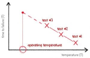
That’s right. Whenever we do ALT, all we try to in basic terms is create a straight line that can then help us estimate the ‘true’ time to failure for our product or system in at use conditions. Ok … there are a couple more things to it than that. But what we are trying to make something like …

We conduct tests where we measure the time to failure (TTF) at various temperatures (T) and try and create this straight line. We then extend the line to the ‘operating’ temperature – and we get our TTF estimate for operating conditions.

Now as with most things in nature – stuff like this rarely makes a beautiful straight line. And that is where Acceleration Factors (AFs) come in. An AF simply tells you how much you accelerate the degradation of your product or system when the temperature increases. For example, increasing temperature by 30 degrees Celsius may have an AF of 2. This means that every day you test your product or device at a temperature elevated by 30 degrees Celsius is equivalent to 2 days of normal usage.

And the AF changes as you go on increasing temperature. Increasing the temperature by 50 degrees Celsius may have an AF of 6.

But how do we get these AFs? Well – we use that model we talked about. And sometimes the right model is not immediately clear. But there is one model that tends to work pretty well – the Arrhenius Model. It looks like this:

$$k=Ae^{\frac{-E_a}{RT}}$$

where k is the rate at which the temperature based reaction is occurring, A is what we call the ‘pre-exponential’ factor, Ea is the ‘activation energy’ of the chemical reaction which is analogous to how much thermal energy is needed to make something happen, R is the ‘Gas constant’ and T  is the temperature in degrees Kelvin.

Yuck. How do you find out these factors and activation energies? Well – you don’t really need to. But what you do need to do in your ALT is conduct multiple tests at multiple temperatures.

I thought you said it’s all about ‘straight lines?’

That’s why you need the model. If you rearrange the model, you can get the equation for our straight line (even if it is a little ugly).

$$\text{ln}(k)=\text{A}-\frac{E_a}{R} \times \frac{1}{T}$$

So if we create a chart. The vertical axis is expressed in terms of …

$$\text{ln}(k)$$

The horizontal axis is expressed in terms of …

$$\frac{1}{T}$$

And then anything that follows the Arrhenius model will create a straight line.

This is great! Remember that k was the rate at which the reaction was occurring? So if failure is occurring twice as fast, then it will failure will occur twice as quickly. So our time to failure (TTF) is simply the inverse of k.

$$k=\frac{1}{TTF}$$

So our straight line equation becomes:

$$\text{ln}(\frac{1}{TTF})=\text{A}-\frac{E_a}{R} \times \frac{1}{T}$$

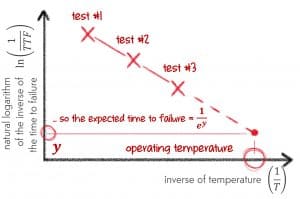
Now this means our straight-line chart above now looks like this:

A chart with these scales on each axis is called an Arrhenius plot – for obvious reasons. Any thermally induced failure mechanism that follows the Arrhenius model will always create a straight line in an Arrhenius plot.

And did you notice the best thing about this! We didn’t need to find out what the constants were in the horrific equation that defines the Arrhenius model. We don’t need to calculate k, A, Ea or R. You simply do multiple ALTs and a straight line will do all the work for you.

But what about temperature cycling?

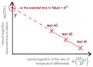
There is another model called the Coffin-Manson model, and the plot we need to make to get our straight line is shown below. I don’t think I need to go into too much detail here, because we are following (at least in principle) the same process we followed for our Arrhenius plot. We just use the model to create a straight line.

But what if we don’t get a straight line?

Good question. What this means is that the underlying model does not describe how temperature affects the failure of your product or system. So – you need to go looking for the right one. There are plenty of models out there, and this article is not long enough to cover all of them! That said, the models we have talked about so far are fairly common in reliability applications.

But how do I know which model to use?

Ok … this question is a little out of sequence. But for a reason.

You can never know with absolute certainty which model works for your product or system. So you have to do multiple ALTs at various temperatures to get your straight line. Even if you know from experience that the Arrhenius model describes the thermal degradation of the adhesive polymer in your power supply – you can never be sure what those constants and parameters that define the model actually are.

You always need to validate with that straight line.

How accurate are the results?

This is where you will need software to help. There are several packages out there that can create your Arrhenius and Coffin-Manson plots for you. And – they can also put confidence bounds on the results. These confidence bounds are the outputs of a messy, statistical framework that takes into consideration how many tests you have run and how well your test data fits the straight line.

But in many cases, we are after a point estimate. And you can often do this by hand!

What if I need help?

Feel free to reach out and ask us at any time. But there are also plenty of really good books out there. Wayne Nelson’s Accelerated Testing is one of the most widely used texts in the field. But again – never feel afraid to ask for help!

   Ask a question or send along a comment. Please login to view and use the contact form.