Why Weibull? 

What if you don’t have lifetime data??

I searched the Internet for “Why Use Weibull Reliability?” and got 196 hits “similar sites omitted”. Some hits looked like they were generated by Chat GPT. None showed data. None told how to test or use Weibull reliability estimates. Many sell Weibull software. All require lifetime data.

Assuming a continuous, parametric distribution such as Weibull conveniently extrapolates limited, censored lifetimes to estimate MTBF, even though MTBF may be far in the future. Https://en.wikipedia.org/wiki/Weibull_distribution lists many uses for Weibull distributions. A client had me use Weibull to model durations of covered calls!

Some Weibull software compares alternative reliability estimates using goodness-of-fit measures; i.e., Weibull reliability functions vs. other continuous parametric reliability functions. Minitab compares Weibull vs. nonparametric, using the Anderson-Darling test. That made me wonder, why does Minitab estimate Weibull when they have a nonparametric estimate free from assumptions?

Waloddi Weibull said, “Any distribution function can be written in the form 1-EXP[-𝜑(t)].” “The most simple function 𝜑(t) satisfying this condition is…” “a power function (t/a)^b. The only merit of this distribution function is to be found in the fact that it is the simplest mathematical expression of appropriate form…” 

So why not extrapolate nonparametric actuarial failure rate function estimates, a(t), beyond last observed failure at age t_o with power function (t/a)^b splined to a(t_o); i.e., a(t_o)+b(ln(t)-ln(a)) for t>t_o, using regression? The failure rate function a(t)=-dln(R(t)/dt for reliability function R(t)=exp[-(t/a)^b], so Weibull extrapolation of failure rate function is ln((t/a)^b)=b(ln(t)-ln(a)).

Real Failure Rate Functions Don’t Weibull

Figure 1 shows factors that real failure rate functions exhibit: dead-on-arrival (DoA), infant mortality, warranty expiration anticipation phenomenon (WEAP), preventive maintenance (PM), wearout, and attrition or retirement. Incorporating these factors requires nonparametric statistics and actuarial methods for forecasting failures, diagnosing failures, planning maintenance, and stocking spares.

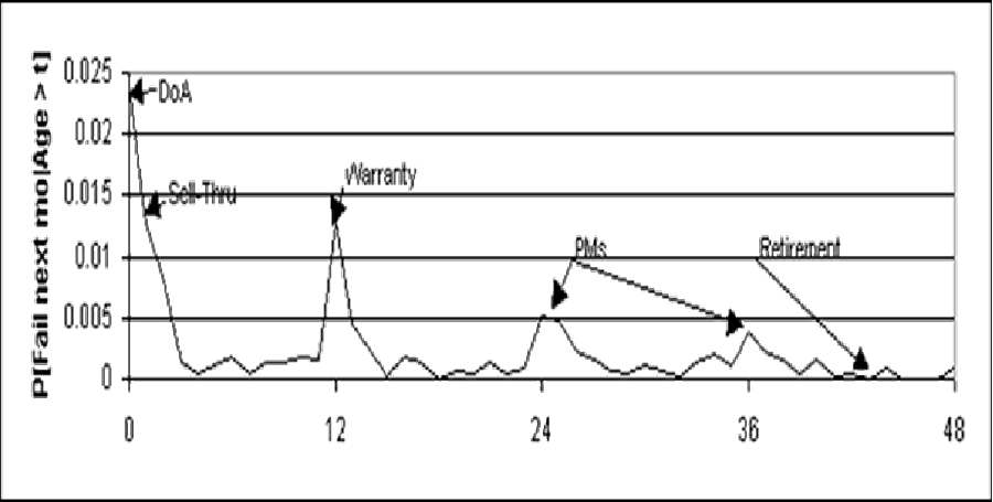
Lab 126 had to fudge Weibull forecasts of warranty returns because their Weibull software didn’t include glitch at warranty.

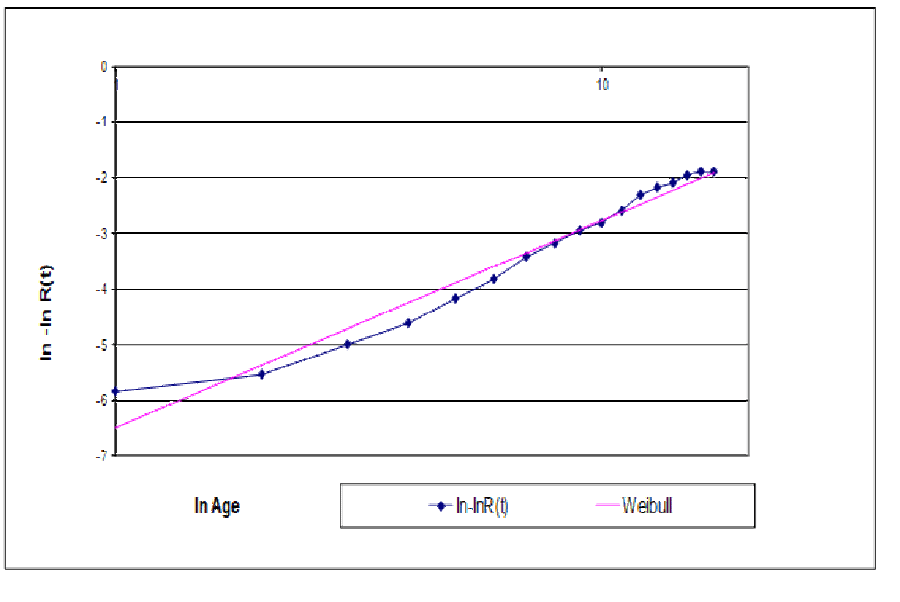
Figure 2 shows a log-log Weibull plot with DoA zero-time failures. Log(1) messes up the plots; that’s when failure occurs on first test cycle or by age 1. It’s easy to estimate a DoA mixture reliability function R(t)=P[Life>t], R(t)=1-P[DoA]-(1-P[DoA])P[Life>t|Life>0] with Weibull P[Life>t|Life>0].

How Can You Estimate Weibull Reliability, Without Lifetime Data?

Periodic ships (sales, production, installed base, etc…) and returns (failures, warranty, complaints, even spares sales) are statistically sufficient to estimate reliability functions, including Weibull, from revenue and service-cost data required by GAAP, plus some work on your part. The methods are least-squares and maximum likelihood. Least squares fits failure rate functions to match observed returns with actuarial hindcasts of returns, for dead-forever or renewal processes.

Gozinto theory converts periodic product installed base ships (cohorts) and returns (failures) counts into parts’ ships and returns counts, by period [https://accendoreliability.com/gozinto-theory-parts-installed-base/#more-417514/]. So you could make Weibull reliability estimates for parts too!

Is the maximum likelihood estimator from ships and returns counts valid? Google AI says, “…max. likelihood estimator is valid only if ships cohort sizes are increasing with time.” That’s false! Increasing ships cohort sizes is a condition for validity of the PAV algorithm (Penalize Adjacent Violators) [Grenander, Marshall and Proschan]. I use max. likelihood and other estimator(s). You could maximize the likelihood function directly as a function of the probability distribution function of service times. Or you could minimize sums of squared errors between observed failures and failure hindcasts (forecasts of what already happened). 

The M/G/infinity (self-service) model of lifetimes says, with Poisson(λ) inputs “M” and service time distribution function G(t), output is Poisson with mean λG(t) [Mirasol]. With nonstationary Poisson inputs at rates λ(t), the M(t)/G/infinity model output is Poisson too! [Eick, Massey, and Whitt, George, https://accendoreliability.com/a-note-on-reliability-estimation-without-life-data/#more-633127/]. The nonparametric maximum likelihood reliability estimator (npmle) likelihood function is a product of nonstationary Poisson distributions with mean E[λ(t-S)]=∫λ(t-s)dG(s), s=[0,t]. (S is the service time random variable with cumulative distribution function G(t).)

Compare Weibull with Nonparametric Estimates?

Statisticians use goodness-of-fit measures to choose among alternative continuous parametric reliability functions: Weibull paper eyeball tests, likelihood ratio tests [Cox, Felthauser], Kolmgorov-Smirnov [George 1997], P-P plots, Anderson-Darling (test for normal distribution? Minitab), correlation,… Mark Felthauser recommends Chi-square. I use likelihood-ratio-test, Akaike-Information Criteria (AIC), Kullback-Leibler divergence (relative entropy in bits), and P-P plots to compare nonparametric vs. Weibull reliability function estimates. 

Table 1 is some example lifetime data in the form of a Nevada table. The “Ships” column lists monthly cohort sizes. The body of the “Nevada” table counts monthly failures from each cohort. The bottom row totals are monthly failures, without knowledge of which cohort they came from.

	Ships	Jan	Feb	Mar	Apr	May	June
Jan	5357	3	6	5	4	1	8
Feb	4222		7	9	12	23	16
Mar	2345			2	13	4	23
Apr	6132				4	8	12
May	2456					2	10
June	??						??
Totals	20512+??	3	13	16	33	38	69+??

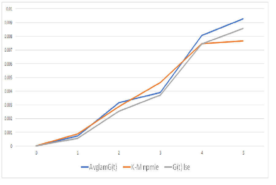
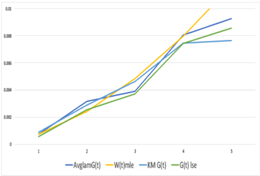
The npmle from the “Ships” cohorts and the failure counts, in the body of the Nevada table, is the Kaplan-Meier estimator. The npmle from ships and returns counts in the bottom row uses direct maximization of the likelihood function. The PAV algorithm didn’t work, because of nonstationarity of the ships process [George 1974]. Figure 3 shows the estimators from ships and returns agree pretty well with the Kaplan-Meier npmle even though returns counts contain less information than failures by cohort in the body of the Nevada table 1.

Figure 3 compares alternative nonparametric distribution function estimates with lifetime data (K-Mnpmle) vs. with average ships and monthly returns data: “AvglamG(t)” and “G(t) lse”. The estimates without lifetime data assumes ships and returns are Poisson inputs to and outputs from an M/G/Infinity self-service system. (Thanks to Mike Johanns who observed that Apple computer lifetimes could be regarded as service times in an M/G/Infinity system [circa 1980]. He made me do a literature search and the only hit was my own paper [George 1973]!)  

How Do People Estimate Weibull?

From lifetime data, perhaps censored, maximize the likelihood function  ∏w(t)^r(t)(1-W(t))^s(t)C(r(t),s(t)) for t=1,2,… up to age of oldest failure… The product is over failure times t, with numbers of failures r(t), and survivors s(t), where w(t) is the discrete Weibull probability distribution function (pdf) w(t;… )=W(t;…)-W(t-1;…), W(t,…) is its cumulative distribution function (cdf), and C(.,.) is the binomial combination function [Cohen, Felthauser, and many others]. Software does it: Reliasoft, Relyence, JMP, SuperSmith, Minitab, R, SAS, and others. Some use regression from lifetime data plotted on Weibull reliability paper using slope and intercept of linear regression line. Regression uses least-squares. Least squares goodness-of-fit to Kaplan-Meier nonparametric reliability from lifetime data is another way to estimate Weibull parameters. (Kaplan-Meier is a maximum likelihood estimator.)

Assuming Weibull makes reliability extrapolation convenient. The Weibull reliability function R(t)=Exp[-(t/a)^b] for t=0 to infinity regardless of limited or censored lifetime data. Extrapolation of nonparametric failure rate function estimates provides alternatives to Weibull assumption: regression of failure rate functions depending on data subsets, incorporation of future events such as preventive maintenance, attrition, retirement, wearout, and end-of-life. Assuming Weibull provides variances of Weibull parameter estimates, but doesn’t account for correlations among parameters or among reliability estimates at different ages.

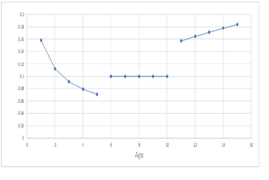
Weibull analyses often provide separate parameter estimates for infant mortality, constant failure rate, and wearout. Try graphing Weibull infant mortality, constant, and wearout Weibull failure rate function estimates (figure 4). You really should make a failure rate function estimates with splined segments [Ferrari]! Good luck with estimating Weibull mixtures with variable failures in each mixture segment [https://accendoreliability.com/failure-rate-classification-for-rcm/#more-499494/]. For help with splines, see paper on B-Splines [Oirov et al.].

Use Lifetime Data to Estimate Weibull Parameters?

Weibull estimation required lifetime data, perhaps censored, until now. Due to the popularity of Weibull analyses, I relented and prepared a Google sheet (“WeiLSE”) that does Weibull estimation, without lifetime data, using least squares, [https://docs.google.com/spreadsheets/d/1eXJtJlUVBL5eJGf_aVDlDnDI8YEznXVA-OY9EQUT5dg/edit?usp=sharing/]. I couldn’t find an optimization program that works in Google Sheets on this problem. So download WeiLSE into Excel if you want to change the data and re-solve using Excel’s Solver.

Goodness-of-Fit Measures for Different Distributions

• Least squares formula is ∑[(G(t) -W(t))²] or chi-square ∑[(G(t)-W(t))²/G(t)]. G(t) could be the nonparametric Kaplan-Meier cumulative distribution function or that from ships and returns, and W(t) could be the Weibull cumulative distribution function estimate. 
• Kullback-Leibler divergence (entropy) is ∑[g(t)Log₂(g(t)/w(t))] (bits) and the pdf g(t) is the Kaplan-Meier pdf or that from ships and returns vs. w(t) the Weibull pdf. (I used Log base 2 so Kullback-Leibler divergence is in bits.)
• AIC Akaike Information Criterion is 2k-2lnL: k is number of parameters estimated; 5 or 6 (ages) for Kaplan-Meier and 2 for the Weibull parameters. This applies to maximum likelihood estimates only (2lnL).
• P-P plots, Weibull probability paper, regression SSE (Sum of Squared Errors), or chi-square.

Table 2 shows goodness-of-fit measures (KLDiv, SSE, Chi-Square, and AIC), nonparametric Kaplan-Meier estimator vs. Weibull estimator from the data in table 1. Kullback-Leibler divergences “KLDiv” Kaplan-Meier vs. Weibull LSE and MLE = 0.00065 and 0.0045! So SSE and Chi-Square estimates fit better (smaller) in terms of entropy or information (bits) and squared error(s)!

Method\Measure	KLDiv	SSE	Chi-Square	AIC
LSE	0.00065	5.57E-06	0.00076	N/A
MLE	0.0045	1.38E-05	0.0033	58.15

What if You Don’t Have Lifetime Data?

Ships’ cohort sizes (column 2 of table 1) and returns (bottom row of table 1) are statistically sufficient to make nonparametric estimates of distribution functions. Assuming an M/G/infinity self-service system model; outputs have Poisson distributions with mean E[λ(t-S)], where S has the service time distribution G(t). Use observed returns and average ships every month in the likelihood function ∏POISSON(returns, Avg(Ships)*G(t), FALSE) t=1,2,…. This seems like a handy way to check validity of npmle of nonstationary M(t)/G/infinity model and estimate of service time distribution: 1. Check G(t) estimate is a legitimate distribution function. 2. Check Poissonness of the ships process. Google sheet does maximum likelihood PAV algorithm for nonparametric estimation assuming M(t)/G/Infinity self-service system with lifetime distribution G(t), under a condition on cohort sizes [https://docs.google.com/spreadsheets/d/1fb_pjwygp_2CUeayNEV4PAX6wyR8sdWqPr76qeJ_n4I/edit?gid=0#gid=0/].

The likelihood function is ∏POISSON(returns(t), λG(t), FALSE), t=1,2,… up to the number of cohorts or ships, when ships are Poisson in M/G/infinity system. That Google sheet uses the PAV algorithm if λ is constant or increasing and Excel’s Solver if λ is more variable. If ships are a nonstationary Poisson process, then test for an M(t)/G/Infinity process, with nonstationary Poisson outputs. It’s impossible to disprove nonstationary Poisson process M(t) from samples for each age t of size one.

	Ships	Returns	M/G/Infinity	M(t)/G/Infinity
Jan	5357	3	0.000731	0.000560
Feb	4222	13	0.003169	0.003079
Mar	2345	16	0.0039	0.006823
Apr	6132	33	0.008044	0.005381
May	2456	38	0.009263	0.015472
LNLikelihood			-4.91613	-4.91613

In 1991 at Apple Computer, I was searching software libraries for optimization programs for maximum likelihood estimation. The NAG library programs didn’t work very well for non-smooth functions. I mentioned that to Dan Fylstra’s brother Dave who said, “Give Dan’s Excel Solver a beta test.” Solver accommodated messy functions such as discrete pdfs, https://www.solver.com/frontline-systems-company-history/ [GRG2 program by Leon Lasdon and Allen Waren]. I used Solver to estimate the reliability of all Apple’s products and their service parts, and…(long story, maybe later).

Weibull Estimation Without Lifetime Data

Estimate Weibull distributions, without lifetime data, using least squares to minimize sums of squared differences between observed returns and hindcasts of returns, Jan.-May. Estimate nonparametric and Weibull using Kaplan-Meier, maximum likelihood, and least squares Weibull fit to Kaplan-Meier, using Jan-May data. Least Squares minimizes ∑[(returns-hindcasts)²].

Some people call |returns-hindcast| “prediction error”: hindcasts are predictions of already observed events based on a model. A hindcast is either an actuarial forecast of (already observed) returns in each period t, ∑a(s)*survivors(t-s) or ∑g(s)*ships(t-s), s=0,1,…,t, where g(t-s) is pdf of G(t) and a(t-s) is its actuarial failure rate function. Minimize the sum of prediction errors squared ∑(returns-hindcasts)² over all nonnegative g(s) or a(s), as long as ∑g(s)<=1. Use Excel’s SUMXMY2(returns, hindcasts) function and Solver for minimization. Least squares is used by linear regression on Weibull paper (or equivalent) to estimate Weibull parameters.

Likelihood Ratio Test, Without Lifetime Data

Compare nonparametric vs. Weibull distribution estimates using Likelihood Ratio test of hypotheses:

Ho: Nonparametric estimate could have come from same population distribution as Weibull vs.

Ha: Weibull doesn’t look likely from ships and returns count. 

Thanks to Mark Felthauser for referring me to David Cox’ suggestion for comparing distribution estimates using likelihood ratio tests. Cox and Mark use L(Weibull)-L(npmle)-E[L(Weibull)-L(npmle)], where expectation E[.] uses the npmle for computing. Dividing that test statistic by its variance yields an approximately normal distribution.

I learned the likelihood ratio test from Jerzy Neyman; the test statistic is -2LN(L(Weibull)/L(npmle)). That’s equivalent to Mark’s LN(L(Weibull))-LN(L(npmle)). The likelihood ratio test statistic has approximately Chi-square distribution (asymptotically). P-values in table 4 are probabilities of Chi-square larger than likelihood ratio test statistic. Table 4 values 8.546 (9.923) come from M/G/infinity and nonstationary M(t)/G/infinity models. Small Chi-square p-values reject Ho: nonparametric and Weibull could have come from same population. Reject Ho.

Compare Kaplan-Meier reliability function estimate (with lifetime data) vs. the nonparametric vs. to Weibull mle and lse. (mle vs mle and lse vs lse). Use the Kullback-Leibler divergence, ∑p(t)Log(p(t)/q(t),2), over the age range t=Jan-May. Log base 2 gives K-L Divergence in bits. Kaplan-Meier vs. Npmle vs. Weibull = 0.0976 (0.0912+0.0064); Kaplan-Meier vs Nplse vs Weibull = 0.1354 (0.0126+0.0094) MLE gets more information than LSE.

Distribution	Log Likelihood	DoF	ChiSq P-value
Nonparametric	-4.96	5
Weibull	-7.38	2
LR Test statistic	8.546 (9.923)	5?	12.9% (9.9%)
LR Test statistic	8.546 (9.923)	3?	3.6% (1.9%)

Why Weibull? Nonparametric Fits Ships and Returns Data Better!

Even without lifetime data, you can make nonparametric reliability function estimates, confidence bands, actuarial forecasts, and their distributions, without unwarranted assumptions. Ships (cohorts) and returns (failures) counts can be found underlying revenue and service costs in data required by GAAP, with a little work! Lifetime data costs more than ships and returns counts (free data plus your work). And you could estimate parts’ reliability too, using bills-of-materials. 

Good luck if you get different Weibull shape parameter estimates for bathtub failure rate(s): for infant mortality, for constant, and for wearout. Mixture distributions are hard to estimate with sparce lifetimes in each age interval. It’s hard to spline Weibull failure rates. Please refer to my RCM article for splining Weibull failure rate line segments, https://accendoreliability.com/?s=RCM+classification/.

Why estimate Weibull from a sample of lifetime data when you can make nonparametric estimates and Weibull from population data required by GAAP. I’ll help. Send data.

Voices from the Past

Rupert Miller said, in comparison with Weibull, “…the asymptotic efficiencies [ratio of variances] of the Kaplan-Meier estimator [nonparametric, right-censored] are low, especially for high censoring proportions or for surviving fractions that are close to one or zero. Low efficiencies for high surviving fractions…are not a cause for worry because the variances of both the Kaplan-Meier estimator and the maximum likelihood [Weibull] estimator are small and the surviving fraction is accurately estimated.”

1999: Ralph Evans, Managing Editor of IEEE Transactions on Reliability, said, “Field-data are largely garbage. I believe they deserve all the negative thinking possible.” Imagine 600Gb worth. I countered and Ralph replied, “True field-data are wonderful-much better than fancy equations. Unfortunately, they are very difficult to get. Thus data from the field are largely garbage because they do not represent what really happened.”

Weibull Might Have Said…

It is gratifying to see the developments in statistics and reliability since I died on October 12, 1979, particularly the use of the Fréchet distribution that I described in my 1939 and 1951 papers. It is now widely referred to as the Weibull reliability function. It seems to be overused in some subject areas, without careful reasoning and justification. It is, however, a better representation of reliability than a constant failure rate. 

It is not gratifying to see how the author has abused Weibull statistics in an earlier article [“What MTBF Do You Want?”] to recommend mixing bad, infant mortality products with good products to achieve a specified MTBF according to the Weibull mixture mean, E[Life] = a𝚪(1+1/beta₁)/eta₁+(1-a)𝚪(1+1/beta₂)/eta₂ where 0<a<1 and beta₁<1<beta₂. Sadly, that author persecutes engineers who use Weibull software without first plotting and understanding their data. That author uses my own words to justify the power law extrapolation of nonparametric failure rate functions. 

Engineers must decide whether to extrapolate nonparametric failure rates or use the Weibull failure rate function beyond the age of the oldest observed failure. Engineers must make sure that anomalies in data collection do not corrupt parameter estimates and forecasts before accepting the Weibull or other extrapolations.

Except for extrapolating actuarial failure rates for quantifying uncertainty, the author’s paper contains nothing new. In fact actuarial failure rates and forecasts predate my 1939 paper. As I wrote in my 1951 paper, “the Weibull distribution has no theoretical basis…there are-with very few exceptions-the same objections against all other distribution functions… It is believed that in such cases the only practicable way of progressing is to choose a simple function, test it empirically, and stick to it as long as no better is found.” 

References

Robert Abernathy, “The New Weibull Handbook Fifth Edition, Reliability and Statistical Analysis for Predicting Life, Safety, Supportability, Risk, Cost and Warranty Claims,” Spiral-bound, Amazon, November 1, 2006

Jim Brenneman, “Weibull? Or is There a Better Fit Using Other Distributions?” ASQ RRD Webinar, https://asqrrd.org/, July 2025

A. Clifford Cohen, “Maximum Likelihood Estimation in the Weibull Distribution Based On Complete and On Censored Samples,” Technometrics, Vol. 7, No. 4 November, 1965

David R. Cox, “Tests of Separate Families of Hypotheses,” Proceeding of the Fourth Berkeley Symposium, Vol. 1, pp. 105-123, 1961

David R. Cox, “Further Results on Tests of Separate Families of Hypotheses,” J. Royal Statistical Society, Series B, Vol. 24, pp. 406-424, 1962

S. G. Eick, W. A. Massey, and W. Whitt, “The Physics of the M(t)/G/Infinity Queue,” Ops. Res. , 41, 731-742, 1993

Mark Felthauser, “A Comparison of Particle Size Models Using the Method of D. R. Cox,” Colorado State Univ. thesis, Spring 1988

Andre-Michel Ferrari, “Failure Free. How Come?”, https://accendoreliability.com/failure-free-how-come/, Nov. 2025

U. Grenander, “On the Theory of Mortality Measurement,” Skandinavisk Aktuarietidskrift, 39, parts I and II, pp. 70-96 and 125-153, 1956

Semion Gringrinovich, “Why Weibull Distribution is Most Common Used in Engineering,” https://accendoreliability.com/why-weibull-distribution-is-most-common-used-in-engineering/

Leon Lasdon and Allen Waren, “Nonlinear Programming Packages,” https://camo.ici.ro/nonlin/grg2.htm/

Albert W. Marshall and Frank Proschan, “Maximum likelihood estimation for distributions with monotone failure rate,” Annals of Math. Statist., 36, 69-77, 1965

Rupert G. Miller, Jr. “What Price Kaplan-Meier?” Biometrics, Vol. 39, No. 4, pp. 1077-1081, Dec. 1983

Minitab Blog Editor, “Why the Weibull Distribution is Always Welcome,” https://blog.minitab.com/en/blog/understanding-statistics/, March 2013

Noel Mirasol, “The Output of an M/G/Infinity Queuing System is Poisson,” Operations Research, Vol. 11, No. 2, pp. 282-284, Mar.-Apr., 1963

Quanterion.com, “The Many Benefits of Weibull Analysis”

Tserenbat Oirov, Gereltuya Terbish, and Nyamsuren Dorj, ”B-spline Estimation for Force of Mortality,” Mathematics and Statistics, Vol.9, No.5, pp. 736-743, DOI: 10.13189/ms.2021.090513, 2021   

W. Weibull, “A statistical distribution function of wide applicability”, J. Appl. Mech.-Trans. ASME 18 (3): 293–297, 1951 

References by George

“Estimation of a Hidden Service Distribution of an M/G/Infinity Service System,” Naval Research Logistics Quarterly, pp. 549-555, Vol. 20, No. 3, co-author A. Agrawal, September 1973

“Maximum Likelihood Estimation of Weibull Parameters With a Worksheet,” Apple Computer, Oct. 1987

“A Note on Estimation of a Hidden Service Distribution of an M/G/Infinity Service System,” Random Samples, ASQC Santa Clara Valley, June 1994

“What MTBF Do You Want?” ASQC Reliability Review, Vol. 15, No. 3, pp. 23-25 https://accendoreliability.com/what-mtbf-do-you-want/#more-598997/, Sept. 1995

“Kolmgorov-Smirnov Two-Sample Test with Censored Data. (To the man with a hammer, everything looks like a nail.)”ASQ Reliability Review, Vol. 17, No. 1, March 1997

“Progress in USAF Engine Logistics?” https://accendoreliability.com/progress-in-usaf-engine-logistics/#more-633124/, May 2025