
Imagine observing inputs and outputs of a self-service system, without individual service times. How would you estimate the distribution of service time without following individuals from input to output? The maximum likelihood estimator for an M/G/Infinity self-service-time distribution function from ships and returns counts works for nonstationary arrival process M(t)/G/Infinity self-service systems, under a condition. A constant or linearly increasing arrival (ships) rate satisfies the condition. If you identify outputs by failure mode then you could estimate reliability by failure mode or quantify reliability growth, without life data.
Reliability Estimation Without Life Data?
Except for high-cost or repairable products, there is little incentive to record when returns or failure were shipped, so there is no time-to-return data from which to estimate reliability. Since 21 CFR Part 821, pacemakers have been tracked by serial number from implant to failure. Medtronic used to publish pacemaker sales and failure counts and their reliability estimates from lifetime data. I made nonparametric reliability estimates from their pacemaker sales and failure counts. Our estimates agreed, and I sent them to Medtronic. Medtronic quit publishing sales, failure counts, and reliability estimates from their pacemaker lifetime data!
Product lives could be regarded as service times of an M/G/Infinity self-service system. System inputs are “ships”: sales, installation, or shipments of a product, by accounting interval. System outputs are “returns”: complaints, failures, repairs, replacements, spares ships or returns of parts.
Larry Baxter derived a reliability function estimator from ships and renewals data, when all the ships occurred at the start [Baxter]. Unfortunately ships occur every month, and returns come back without a clue about how old they are.
Ships and returns counts provide statistically sufficient data to estimate products’ and parts’ reliability functions. A reliability function is one minus the service-time distribution function G(t) of an M/G/Infinity self-service system, because ships “serve” for a random time [George and Agrawal].
The output from an M/G/Infinity service system is a Poisson process with mean rate λG(t) where λ is the Poisson mean input rate [Mirasol]. The Poisson output mean rate λG(t) is analogous to the failure rate function of a time-to-failure random variable. Ulf Grenander and later Albert Marshall and Frank Proschan derived the Pool Adjacent Violators (PAV) nonparametric maximum likelihood estimator (npmle) of an increasing failure rate function. The npmle of λG(t) gives the npmle of G(t) by dividing λG(t) by the input rate λ, because, under reasonable conditions, a function of an npmle is also an npmle.
Applications sometimes violate conditions to represent returns as output from a M/G/Infinity system. Ships are seldom a stationary process.
Extension to Nonstationary Ships
There are alternative methods to handle nonstationary shipping rates [George], but npmles of reliability functions are desirable for their properties and require no unwarranted distribution assumptions. The reliability function npmle could be valid when the input Poisson process rate λ(t) is nonstationary.
Theorem 1 of [Eick, Massey and Whitt] says, “The departure process (of an M(t)/G/Infinity system) is a Poisson process with time dependent output rate δ(t)=E[λ(t-S)].” S is the service-time random variable, and the expected value E[λ(t-S)] ∫λ(t-s)dG(s) integrated from s=0 to t. λ(t-S) is the ships input rate at time t-S. If E[λ(t-S)] is nondecreasing, then the npmle of a nondecreasing failure rate function may be used to estimate E[λ(t-S)] and G(t).
For example, suppose the Poisson rate is a constant λ. Then, E[λ(t-S)]=∫λ*dG(s)=λ*G(t)) and is nondecreasing because G(t) is a distribution function, nondecreasing in age t. For another example, suppose the Poisson rate λ(t) is a linearly increasing function, λo+λ*t, for t ≥ 0. Then, E[λ(t-S)] = ∫λo+λ*(t-s)dG(s) = λ*(λo+λ*G(t)) and is nondecreasing.
The npmle of E[λ(t-S)] puts mass at a subset of M(t)/G/Infinity departure times (return times in the reliability context). Those masses may be solved for the discrete npmle of the probability density function g(t). The npmle of E[λ(t-S)] with linearly increasing λ(t) is the npmle of λo +λ[G(t) – G(0) – ∑u*g(u)], where the sum from u>0 to t runs over the set of return times, u, at which the npmle of E[λ(t-S)] puts mass. This discrete function can be solved for G(t) at jumps. The npmle of G(t) is constant elsewhere.
Suppose the first return occurs at time t1 > 0 and the npmle puts mass g(t1) at t1. Then the npmle of G(0) is 0 and the npmle of g(t1) is (g(t1)-λo)/(λ(λ-t1)) if nonnegative. Remaining values of g(u) may be solved recursively for values of u where the npmle puts mass.
An Example of Grouped Data
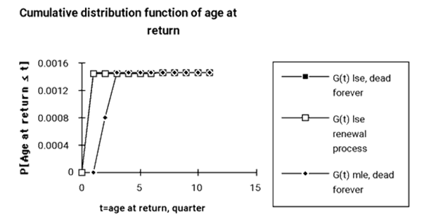
Table 1 shows the numbers of ships and returns by quarter for a product. Figure 1 shows the npmle and least squares estimates (nplse) [George 2008] of the cumulative distribution function G(t) of ages-at-returns. There is not enough data to test whether the nonstationary ships process is Poisson. The condition for using the npmle with a nonstationary Poisson input is satisfied for all observed times. Table 2 lists increasing values of E[λ(t-S)].
Nonparametric least squares estimators (nplse) are computed under two assumptions: returns are from dead forever products or products that undergo renewal. Both estimators agree on G(t) after the third quarter (figure 1). The nplse puts all failure probability in the first quarter, and the npmle divided it between the third and fourth quarter.
Suppose the input rate λ(t) doesn’t keep up with the output rate, so ships < returns. This violates the conditions for the maximum likelihood estimator [George 1993]. The returns may be a renewal or other kind of replacement process and need a different model of ships and returns such as a renewal process shown in figure 1 [Tortorella, George 2008].
Table 1. Ships and returns data
| Quarter | Ships | Returns |
| 1 | 892 | 0 |
| 2 | 64537 | 52 |
| 3 | 352133 | 937 |
| 4 | 851677 | 2826 |
| 5 | 1452959 | 3913 |
| 6 | 2469820 | 4175 |
| 7 | 3815927 | 7975 |
| 8 | 5288164 | 9326 |
| 9 | 6837147 | 6962 |
| 10 | 8268514 | 9436 |
| 11 | 6001803 | 5838 |
Table 2. E[λ(t-S)] should be nondecreasing for npmle
| Age at return, quarters | E[λ(t-S)] |
| 1 | 0 |
| 2 | 0 |
| 3 | 0.7187 |
| 4 | 52.58 |
| 5 | 325.6 |
| 6 | 914.6 |
| 7 | 1723 |
| 8 | 2932 |
| 9 | 4676 |
| 10 | 6735 |
| 11 | 8938 |
What Happens in Steady State?
Information from the M/G/Infinity output dwindles as it approaches steady state. Eventually G(t)->1 and output rate λ*G(t)-> λ, so outputs have no information about the service time distribution. Furthermore, a nonstationary Poisson mean input rate function λ(t) could invalidate the condition for the PAV (Pool Adjacent Violators) algorithm for the maximum likelihood estimator of λ(t)G(t). Ships and returns counts can be derived from sales, warranty, repair cost, or spares sales data required by generally accepted accounting principles. But, I’ve seen data where period ships were negative for unknown reasons: product returns, data entry errors, other?
When ships data look suspiciously nonstationary, I’ve used moving averages for λ(t). As I recall, the moving average is the maximum likelihood estimator of the ship rate function.
What if There are Multiple Failure Modes, Product Changes?
If the Poisson outputs from an M(t)/G/Infinity self-service system are categorized by failure mode or COVID-19 cases are categorized by variant, then it is possible to estimate reliability or survival functions conditional on mode or variant. It’s tricky, because observed failures, recoveries, or deaths become mixtures of variants.
If inputs and outputs were also categorized by failure mode or COVID-19 recovery, death, or variant, then the PAV algorithm could be used separately on each category. If not, it is possible to estimate “survival” functions for both COVID-19 time to death and time to recovery from case, recovery, and death counts, because categorized outputs have Poisson distributions conditional on category. Maximum likelihood and least squares both work to estimate conditional reliability or survival functions, including Paretos or Case Fatality Ratios in the optimization (figure 2). In the reliability context, it is possible to estimate reliability functions, from ships and returns counts, the latter categorized by failure mode.
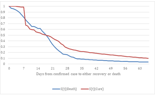
COVID-19 variants seem to have become less lethal, but survival functions estimates for successive variants have to account for deaths and recoveries from earlier variants. The same methods work for quantifying product reliability growth due to product changes, not MTBF growth as in [Duane, AMSAA Crow]. Maximize the log likelihood function or minimize the sum of squared errors between observed failure mode counts and actuarial hindcasts ∑a(s)*n(t-s) of past failure mode counts, simultaneously, as functions of the conditional distribution functions G(t|category) (likelihood) or conditional actuarial rates a(s|category)=
(G(t| category)- G(t-1|category)/G(t| category).
If you would like examples of multivariate survival function or reliability function estimation, without life data, ask or send data.
References
L. A. Baxter, “Estimation from Quasi Life Tables,” Biometrika, Vol. 81, No. 3, pp. 567-577, Aug., 1994
L. H. Crow, “Methods for Assessing Reliability Growth Potential,” IEEE Proceedings Annual Reliability and Maintainability Symposium, pp. 484-489, 1984
J. T. Duane, “Learning Curve Approach To Reliability Monitoring,” IEEE Transactions on Aerospace, Vol. 2, pp. 563-566, 1964
S. G. Eick, W. A. Massey, and W. Whitt, “The Physics of the Mt/G/Infinity Queue,” Ops. Res. , 41, 731-742, 1993
L. L. George, “Estimate Reliability Functions Without Life Data,” ASQ Reliability Review, 13, 21-25, 1993
L. L. George and A. Agrawal, “Estimation of a Hidden Service Distribution of an M/G/Infinity Service System,” Naval Research Logistics Quarterly, vol. 20, pp. 549-555, 1973
L. L. George, “Renewal Estimation Without Renewal Counts,” ASQ Tech Briefs, Vol. 2, 2008
U. Grenander, “On the Theory of Mortality Measurement,” Skandinavisk Aktuarietidskrift, 39, parts I and II, pp. 70-96 and 125-153, 1956
Albert W. Marshall and Frank Proschan, “Maximum likelihood estimation for distributions with monotone failure rate,” Annals of Math. Statist., 36, 69-77, 1965
Noel Mirasol, “The Output of an M/G/Infinity Queuing System is Poisson,” Operations Research, Vol. 11, No. 2, pp. 282-284, Mar.-Apr., 1963
Mike Tortorella, “Life Estimation from Pooled Discrete Renewal Counts.” in: Jewell N.P., A.C. Kimber, Lee ML.T., Whitmore G.A. (eds) Lifetime Data: Models in Reliability and Survival Analysis. Springer, Boston, MA, 1996

Leave a Reply