This is a non-parametric test to compare ranked data from three or more groups or treatments. The basic idea is to compare the mean value of the rank values and test if the samples could are from the same distribution or if at least one is not.
The null hypothesis is the data from each group would receive about the same mean rank score. We are comparing rank values, not the actual values.
Assumptions
- The data may be any distribution or an unknown distribution.
- The data should be continuous and suitable for rank ordering.
- The observations are mutually independent.
Analysis Steps
- Set up the hypothesis test
The null hypothesis, Ho: The k distributions are identical given k different sets of measurements.
The alternative hypothesis, Ha: At least one of the k distributions is different than the others.
Note: the test does not indicate which group or how many are different.
- Determine the Test Statistic
The test statistic is calculated with
$$ \large\displaystyle H=\frac{12}{{{n}_{T}}\left( {{n}_{T}}+1 \right)}\sum\limits_{i=1}^{k}{\frac{T_{i}^{2}}{{{n}_{i}}}-3\left( {{n}_{T}}+1 \right)}$$
Where ni is the number of measurements from sample i,
nT is the total sample size across of sets of measurements,
and, Ti is the sum of the ranks in sample i after assignment of ranks across the combined sample.
- Determine the Rejection Region
Given a confidence level, C, let α = 1 – C. Reject Ho if H exceeds the critical value of χ2 for a = α and df = k – 1
- Calculate corrected H, H’, if there is a large number of ties in the data, use
$$ \large\displaystyle H’=\frac{H}{1-\left[ \sum\nolimits_{j}{\frac{\left( t_{j}^{3}-{{t}_{j}} \right)}{\left( n_{T}^{3}-{{n}_{T}} \right)}} \right]}$$
where ti is the number of measurements in the nth group of tied ranks.
Sample Problem
Let’s say we are exploring the service life a specific bearing location across three machines to determine if the time to failure is the same for each machine or not.
We know the time to failure data is not normally distributed (most likely Weibull distribution yet we do not have enough data from each machine to determine the Weibull distribution parameter estimates.)
We have the following time to failure data (in months)
| Machine A | Machine B | Machine C |
|---|---|---|
| 12 | 14 | 9 |
| 19 | 20 | 14 |
| 26 | 14 | 11 |
| 23 | 16 | 8 |
| 20 | 22 | |
| 29 |
Set up the Hypothesis Test
Ho: There is no difference in bearing time to failure across the three machines.
Ha: At least one machine bearing lifetime is different than the others.
Compute the Test Statistic
- Combine the data in rank order and assign ranks.
| Combined Data | Rank | Machine |
|---|---|---|
| 8 | 1 | C |
| 9 | 2 | C |
| 11 | 3 | C |
| 12 | 4 | A |
| 14 | 6 | C |
| 14 | 6 | B |
| 14 | 6 | B |
| 16 | 8 | B |
| 19 | 9 | A |
| 20 | 10.5 | A |
| 20 | 10.5 | B |
| 22 | 12 | B |
| 23 | 13 | A |
| 26 | 14 | A |
| 29 | 15 | A |
For ties, the rank is the average of the span of ranks the group would occupy. For example, in the data, there are three bearings that failed after 14 months. The three values would receive ranks of 5, 6, and 7, therefore, use the average of the three rank values, or 6 in this case.
- Now, sort the data back in the three groups and determine the average rank value for each machine. The values in parenthesis are the rank value for that measurement.
| Machine A | Machine B | Machine C |
|---|---|---|
| 12 (4) | 14 (6) | 9 (2) |
| 19 (9) | 20 (10.5) | 14 (6) |
| 26 (14) | 14 (6) | 11 (3) |
| 23 (13) | 16 (8) | 8 (1) |
| 20 (10.5) | 22 (12) | |
| 29 (15) | ||
| 65.5 | 42.5 | 12 |
- Compute H
$$ \large\displaystyle \begin{array}{l}H=\frac{12}{15\left( 15+1 \right)}\left[ \frac{{{\left( 65.5 \right)}^{2}}}{6}+\frac{{{\left( 42.5 \right)}^{2}}}{5}+\frac{{{\left( 12 \right)}^{2}}}{4} \right]-3\left( 15+1 \right)\\H=\frac{12}{240}\left( 715.04+361.25+36 \right)-48\\H=7.61\end{array}$$
Note: there are only 5 measurements in ties. In general, a use H’ when there are over half the values involved in ties.
- Determine the Rejection Region
The critical value of the χ2 distribution with α = 0.05 and df = k – 1 = 2. Using a χ2 table we find a critical value of 5.991.
- Conclusion
Since the test statistics is greater than the critical value (in the rejection region) we conclude that at least one of the machines wears out bearings at a different rate than the others.
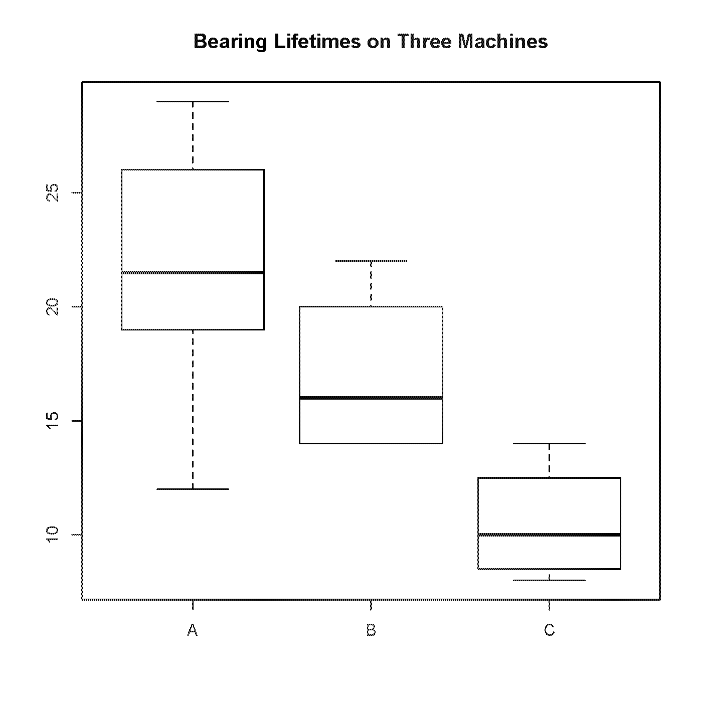
A box plot may provide additional information and is a good way to visualize the data from the three machines.
Related:
Moods Median Test (article)
Levene’s Test (article)
Mann-Whitney U Test (article)

 Ask a question or send along a comment.
Please login to view and use the contact form.
Leave a Reply