
We are well aware of cases when Accelerated Testing is successfully creating by statisticians, here I would like to propose an engineer’s approach.
We have created a new product, there is (is) an order for it (50 products at a price of $200). Can we start manufacturing and delivery? No, we can’t. We are stopped by significant warranty obligations and lack of confidence in the reliability of the product during the warranty period.
This is a typical task with uncertainty.
This case reminds me of the story “Stone Soup”, when we do not have any data:
One day a wandering soldier came into the village. He asked the different
people he met about finding a place to eat and sleep for the night.
“There’s not a bite to eat in the whole county,” they told him. “You better keep moving on.”
But we have to get the result – to develop and implement such a program of reliability verification and improvement of the product, which includes a set of tests and measures to eliminate the causes of detected failures to ensure a successful life cycle of the product.
To me, the «Stone Soup» here is a general method for solving problems with uncertainty called the “worst case” method. It is an objective method.
“Oh, I have everything I need,” he said. “In fact, I would like to make some stone soup to share with all of you.” He pulled a big black cooking pot from his wagon. He filled it with water and built a fire under it. Then, he reached slowly into his knapsack and, while several villagers watched, he pulled a plain gray stone from a cloth bag and dropped it into the water.
The “worst case” indicator is considered to be the maximum of the Life Cycle Cost (LCC) of the product, which includes here:
– the cost of development/improving the reliability of the product
– cost of manufacturing products to fulfill the contract
– warranty costs.
LCC is a random value, so we consider it with a given Confidence Level (hereinafter CL=0,9, i.e. such a value of LCC that with a probability of CL=0,9 will not be exceeded).
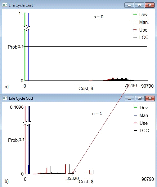
The product contains four Critical Parts with reliability from 0.2 to 1 each (the range of uncertainty of probability of failure-free operation is 0.2…1 for each part). “Worst case” there is an obvious one – it is the smallest reliability of 0.2 for each part (0.2; 0.2; 0.2; 0.2; 0.2). The life cycle cost would be $78230 (Fig.1a), which includes:
– there is no product reliability development/improvement, development cost is $0
– product manufacturing cost is $2650
– warranty cost (the cost of repairs or replacements during the warranty period) is $76380 (CL=0,9) (negative binomial law of distribution of the number of failures for each of the four Critical Parts with probability of failure 0,8 and the number of products 50).
LCC $78230 at a contract price of $10000 is not very favorable business.
“Ahh,” the soldier said aloud to himself, “I do like a tasty stone soup. Of course, stone soup with cabbage is even better.”
Soon a villager ran from his house into the village square, holding a cabbage.
The soldier cut up the cabbage and added it to the pot.
We will carry out reliability development/improvement by means of tests, trying to improve the efficiency of such tests.
We will test one product within the warranty period of 2000 hours (Bernoulli test). If there are no test failures, we will manufacture the products and perform delivery under the contract. If there are test failures, we will redesign the product to eliminate the causes of the identified failures (the cost of manufacturing the redesigned product increases, as a rule).
How do we search for the “worst case” if we do a test? The logic of this search is very simple:
The reliability uncertainty of each Critical Part of the product is from 0 to 1 (in the constraints I set from 0.2 to 1).
– If the reliability of the product is small (about 0), then with a high probability (about 1) a failure will be found in the test, a redesign will be done and a product with high reliability will enter production and operation. This is a “good case”
– if the reliability of the product is high (about 1), then no failures will be found in testing, no redesign will be done, but the product with high reliability will be put into production and operation as well. This is a “good case” too.
– if the product reliability is intermediate between 0 and 1, for example 0.5, then there is a high probability of missing (not finding) a failure in testing, not eliminating its causes and there is a high probability of failures in operation. This is the “bad case”. Therefore, the search for the “worst case” in the range of product uncertainty as a maximum of product life cycle cost is relevant.
When testing one product, the “worst case” life cycle cost of the product is $35320 (Fig.1b):
– development cost is $220
– product manufacturing cost is $3050
– warranty cost is $32920
At a contract price of $10000 this is not a very profitable business either.
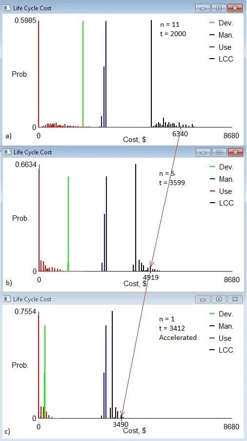
“If we can calculate, we can manage as well”. We can determine and assign such a number of Bernoulli tests (number of samples) to reduce the LCC. For example, when we test 11 products, the “worst case” LCC is $6340 (Fig.3a) with Critical Parts reliability (0.82; 0.84; 0.87; 0.45):
– development cost is $2010
– product manufacturing cost is $3050
– warranty cost is $1320
Further increasing the number of tests does not reduce the LCC because the reduction in warranty costs does not offset the increase in the cost of development.
Often, the cost of testing is too high or the products are unique. For example, aircraft engines. In these cases, we cannot significantly increase the number of tests.
“Any soup needs salt and pepper,” said the soldier, as they began to stir.
Children ran to fetch salt and pepper.
If we add knowledge about the durability distribution laws of the Critical Parts, we can improve test efficiency not only by increasing the number of samples (n), but also by increasing the time of each test (t). To do this, we need to work with the “tails” of the durability distributions. Increasing the test time increases the probability of failures, which makes it easier to find potential failures in the tests.
Experience in testing and operation of similar products and their Critical Parts, knowledge of the failure mechanism allows us to assume types of Critical Part durability distribution laws (Weibull, Lognormal, Normal, etc.) and shape parameter values that are the same for certain failure mechanisms, as a rule. The scale parameters are unknown, generally, but a possible range of their values (uncertainty range) can be determined. Some values of the scale parameter correspond to low reliability values, while others correspond to high values. In out example:
Part 1 – Weibull (1590 – 30000; 2)
Part 2 – Weibull (1740 – 16000; 3.3)
Part 3 – Lognormal (3.135 – 3.96; 0.2)
Part 4 – Normal (1710 – 6000; 0.2 – coefficient of variation)
When testing one product, the best test time is 3599 hours (Fig.2a), which is 1.8 of the warranty period. Further increase of testing time would be advantageous, but it is impossible due to the Time to Market limitation (Time to Market is 0.9 years, testing rate is 4000 hours/year).
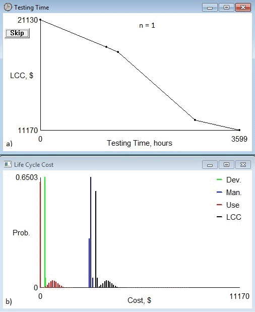
“Worst case” LCC is $11170 (Fig.2b) with the scale parameters of the Critical Parts durability distributions (1590; 3460; 3,894; 5220):
– development cost is $280
– product manufacturing cost is $2850
– warranty cost is $8140.
The best test case where we can control the number of trials n and the duration of each trial t is n=5 and t=3599 hours. In this case, we can provide LCC = $4919 (Fig.3b) with the “worst case” scale parameters of the Critical Parts durability distributions (6000; 5420; 3,465; 3480):
– development cost is $1329
– product manufacturing cost is $3050
– warranty cost is $600.
“You know, I once had stone soup with cabbage and a bit of beef, and it was delicious.”
The butcher said he thought he could find some beef scraps. As he ran back to his shop, other villagers offered bits of vegetables from their own gardens–potatoes, onions, carrots, celery.
Finally, we come to accelerated testing. Forcing of test modes within the limits of invariance of failure mechanisms does not lead to changes in the laws of distribution of critical parts durability and parameters of their shape. In this case, the scale parameters are changed towards durability reduction. The amount of durability reduction is called the Acceleration Factor.
There is an ideal case where each Critical Part depends on its own test mode parameter and can be accelerated independently of the other parts.
We have four test mode parameters R = (r1, r2, r3, r4) per four Critical Parts. The allowable test mode forcing is R = (3.33, 3.33, 1.176, 3.33). The scale parameters of the durability distributions of the Critical Parts depend on the mode parameters inversely proportional to the mode parameters (Scale Parameter in Tests = Scale Parameter in Service/r).
The best test case where we can control the number of trials n, the duration of each trial t and the test mode R is n=1, t=3412 hours and the maximum boosting of the test mode R = (3.33, 3.33, 1.176, 3.33). The acceleration factors on the Critical Parts in this case are AF = (3.33, 3.33, 3.8, 3.33). Such tests provide us with LCC = $3490 (Fig.3c) for the “worst case” scale parameters of the Critical Parts durability distributions (10320; 8260; 3.6; 5310):
– development cost is $290
– product manufacturing cost is $3050
– warranty cost is $240.
In real life, things are not so perfect. Typically, there are few test mode parameters that we can force to accelerate the test, and they give different acceleration for different Critical Parts. For example, increasing the compressed air intake from the Auxiliary Gas Turbine Engine increases the hot part temperature but reduces the axial loads on the rotor. Therefore, determining the most efficient accelerated test mode is a challenging task. Moreover, the efficiency of such accelerated mode may not be sufficient due to existing contradictions. Therefore, we need completely new methods of accelerated testing.
So, we got what we wanted – we developed a program to verify and improve the reliability of a new product, which includes a set of tests and measures to eliminate the causes of identified failures to ensure its successful life cycle. The life cycle cost (with confidence level CL=0.9) was reduced by a factor of 22 – from $78230 when no testing is performed to $3490 when effective accelerated testing is performed.
When the soup was ready, everyone in the village ate a bowl of soup, and it was delicious. The villagers offered the soldier money and other treasures for the magic stone, but he refused to sell it.
All calculations are done by the Life Cycle Simulator program, which is the Stone Soup in our tale.

Leave a Reply