Editing and Contributions by John Healy
Before computers and statistical software, we relied on tables to determine values for common integration problems – the normal distribution in particular. There is no closed form solution for the integral of the normal distribution probability density function, it requires advanced numerical methods to estimate the area under the curve.
The normal distribution has the very pleasant property that it can be normalized. By subtracting the mean and dividing by the standard deviation for each point of in the dataset, the results have a standard normal distribution. The standard normal has a mean of zero and standard deviation of one. This means that if you can estimate the area under the PDF for a standard normal distribution, you can estimate the area under the PDF for a normal distribution with any mean or standard deviation.
Most statistics books, and many reliability engineering books include a standard normal table in an appendix.
The issue is each author may present the table in one of many manners.
There is not a “standard” standard normal table
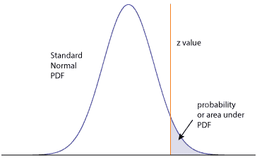
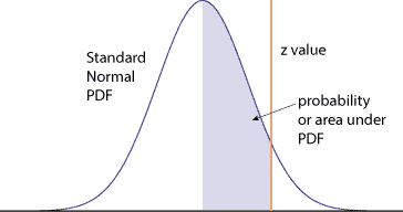
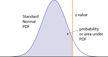
A quick check in a few books found three different layouts for the table. The key is to check the small sketch of the normal curve with a z-value indicated on the x-axis and a shaded in the area under the curve. The shaded area represents the area under the PDF given in the body of the table. It is the probability that a standard normal random variable, Z, is less than or equal to the z-value, between the mean and the z-value or greater than or equal to the z-value.
The left column of all the tables contained the first two digits of the z-value. The top row contained the third digit. Together they represent the z-value. The body of the tables contains four or five digit numbers with values corresponding to the area represented by the shaded region, as the z-value changes.
The CRE primer table has a graphic similar to
Thus the values in the body of the table provide the area under the PDF to the right of the z-value out to positive infinity. Generally, the table will have values from near zero to 0.5 (when the z-value is zero). The higher the z-value the smaller the area.
Let’s try to use this table to find some normal probabilities. For example, if we want to find the probability that a standard normal is greater than 1.45, the table will provide that value directly: P(Z > 1.45) = 0.0735. The total area under the curve is 1. This means that P(Z< 1.45) + P(Z >1.45) = 1 (note that P(Z= 1.45) = 0). As a result, if we want the probability that a standard normal is less than 1.45, we need to subtract the value in the table from 1:
P(Z < 1.45) = 1 – P(Z >= 1.45) = 1 – .0735 =0.9265
If we want the probability that a standard normal is greater than
-1.45, the number “-1.45” cannot be found in the table. Since a normal distribution is symmetric (looks the same on the right and left), the P(Z > -1.45) = P(Z< 1.45). We calculated the P(Z < 1.45) above. As a result we have: P(Z > -1.45) = P(Z < -1.45) = 1 – P(Z> 1.45) = 1 – .0735 = 0.9265
We can also calculate probabilities for a random variable with a nonstandard normal distribution. Let X have a normal distribution with mean 4 and standard deviation 8. Let’s find the probability X is greater than 5 using the table for a standard normal distribution. We know that (X-4)/8 has a standard normal distribution. As a result, we have:
P(X>5) = P((X-4)/8 > (5-4)/8) = P((X-4)/8 > 1/8) = P(Z > .125) = .4503
My trusty statistics book has the following graphic:
Here the value is from the midpoint or mean to the z-value. To the left of the mean is an area of 0.5 from negative infinity to the mean. The table will have values ranging from zero to 0.5. The larger the z-value the higher the value. We can calculate the probabilities for standard and nonstandard normal distribution using this table in a similar manner to what we showed for the table from the CRE primer.
The Juran’s Quality Handbook has the following graphic,
which is the complement of the one found in the primer, and the table provides the area under the curve from negative infinity up to the z-value. The values in the table will range from 0.5 when the z-value is zero or corresponding to the mean up to one. Typically the table will only consider values with positive z-values.
Similar to what we showed for the CRE table, you, with some practice, can find the value you need with some manipulation. A good practice is to draw a small normal curve and shade in the area that you need to solve the problem. Then using the table, find the corresponding area and value.
Some general ideas to keep in mind: The total area under the PDF is one. The value to the left or right of the midpoint, or mean, out to infinity is 0.5. Also, the normal curve is symmetrical, so keep track of the signs of the z-value for the calculations (negative values represent values to the left of the mean). The area above 2.0 z-value is the same as the area below -2.0 z-value.
One note as you prepare for the exam – get used to a specific table and have that table with you during the exam. It only takes simple error to find the wrong answer.
Related:
The Normal Distribution (article)
Point and Interval Estimates (article)
Calculating Lognormal Distribution Parameters (article)


 Ask a question or send along a comment.
Please login to view and use the contact form.
Leave a Reply