A continuous distribution is useful in many statistical applications such as process capability, control charts, and confidence intervals about point estimates. On occasion time to failure, data may exhibit behavior that a normal distribution models well.
The Weibull distribution approximates the normal distribution when the shape, beta, parameter is between 3 and 4. It is common to start exploring time to failure data with the Weibull distribution given its flexibility. If it appears to approximately normally distributed, it may make sense to fit a normal distribution.
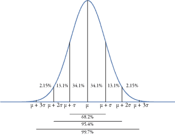
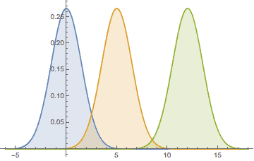
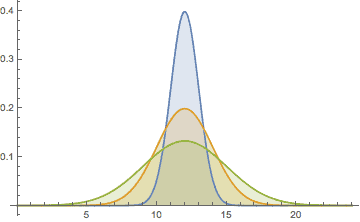
The normal distribution is characterized by the ‘bell shaped curve’. It is symmetrical about the mean and has approximately 68.2% of values within 1 standard deviation of the mean.  The distribution is defined by the mean, μ, and standard deviation, σ. The mean determines the location.
  And the standard deviation the spread.
Probability Density Function, PDF
$$ \large\displaystyle f\left( x \right)=\frac{1}{\sigma \sqrt{2\pi }}{{e}^{-\frac{1}{2}{{\left( \frac{x-\mu }{\sigma } \right)}^{2}}}},-\infty <x<\infty $$
One of the advantages of the normal distribution is due to the central limit theorem. The averages of a sample from a slightly skewed distribution, will be normally distributed. If the distribution for the individuals data is reasonably close to normal, then averaging just a few samples, say 3 or 4 data points, then the averages of the samples will be normally distributed.
For very non-normal distribution it make take 30 or so samples averaged before the group of averages exhibit a normal distribution appearance.
Cumulative Density Function, CDF
The normal distribution PDF can not be integrated implicitly, thus ‘normalize’ the data and use a standard normal distribution to determine the area under the PDF or the CDF values. The transformation is
$$ \large\displaystyle z=\frac{x-\mu }{\sigma }$$
The z value permits entry into the standard normal table to calculate the CDF or Reliability function values. More on the standard normal tables in another article.
Related:
Lognormal Distribution (article)
Chebychev Inequalities (article)
Calculating Lognormal Distribution Parameters (article)
 Ask a question or send along a comment.
Please login to view and use the contact form.
A nice article, as all the other ones. The explanation of the central limit theorem seems to have some words missing? If not, then I don’t get the point.
Hi Peter,
Thanks for the comment and I’ll take a closer look and update the note on central limit theorem. It was in part just a side note as when writing it released it really should be it’s own article and reference here. Sorry any confusion.
Cheers,
Fred
Hi Fred,
Thanks for the succinct article.
Just a quick one: Can I deduct that I have a single failure mode if I have conclusively identified that my times to failure follow the normal distribution closely, i. e. Around 0.98 correlation?
Kindest regards
Khomotso
South Africa
Hi Khomotso,
Not conclusively – fitting a distribution is one thing, doing failure analysis or root cause analysis is another. The data may indicate there is one underlying cause, yet that is only an indication, not evidence.
Cheers,
Fred
PS: glad you found the article and thanks for reading