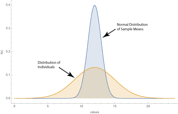
There are two basic ways to consider the central limit theorem. First consider a random variable, X, which has a mean, μ, and variance σ2. If we take a random sample from f(X) of size n and calculate the sample mean, X̄, then as n increases the distribution of the sample means, X̄’s approaches a normal distribution with mean, μ, and variance σ2/√n̄. The original data, X, may have any distribution and when n is suitably large the distribution of the averages will approach a normal distribution.
 A second way to consider the central limit theorem is often used to describe the physical phenomenon behind items that exhibit a normal distribution. Consider the length of a box nail, the final manufactured length depends on the material, cutting and shaping tools, equipment alignment and at a finer level, the material composition, the hardness, and angle of attach of the cutting and shaping tools. With a little effort, one could list many small sources of variation.
When the small perturbations are independent of each other, the sum of those variations tends to approach a normal distribution. Some call this the ‘fuzzy’ central limit theorem.
Fundamental Theorem of Probability
The central limit theorem is one the fundamental theorems of probability. It provides a foundation for most what we study under probability and statistics. In particular, the behavior of even small sample means is the reason X̄ and R control charts work. The averages are normal enough that the calculation of control limits provides meaningful insight into the process stability.
Another fundamental theorem is the law of large numbers which we’ll discuss in another article.
Standard Error of the Mean
Notice that the distribution of the sample means (blue) has less spread then the original data (orange), as apparent in the figure above. Specially the standard deviation of the sample means, σX̄ is
$$ \large\displaystyle {{\sigma }_{{\bar{X}}}}=\frac{{{\sigma }_{X}}}{\sqrt{n}}$$
This of course is estimated by
$$ \large\displaystyle {{s}_{{\bar{X}}}}=\frac{{{s}_{X}}}{\sqrt{n}}$$
The sX̄ and sX sample standard deviations.
The standard error of the mean is used in X̄ and R control charts to determine the control limits, which are plus or minus 3 standard deviation about the mean — that is ± 3 standard errors of the mean.
One final note: The Khan Academy has a sequence of excellent tutorials on this theorem.
Related:
Lognormal Distribution (article)
The Normal Distribution (article)
Laplace’s Trend Test (article)
 Ask a question or send along a comment.
Please login to view and use the contact form.
Leave a Reply