
Introduction
How effective are the repair tasks you conduct on your equipment?
This article looks at quantifying the effectiveness of corrective maintenance, typically an unplanned repair on an asset. Unplanned repairs are undesirable because the asset loses its function and cannot produce what is required often leading to loss of revenue. Yet, this advent is inevitable because assets are subject to degradation over time.
The effectiveness of a repair relates to the condition in which the asset is restored to after a repair. But also how long it will operate until the next repair, Evaluating the effectiveness of the repair will provide the asset operator with a decision making tool. Can we do something different if the repair effectiveness is unsatisfactory? Or do we have to replace the asset as it is failing too frequently?
Repairable versus non-Repairable systems
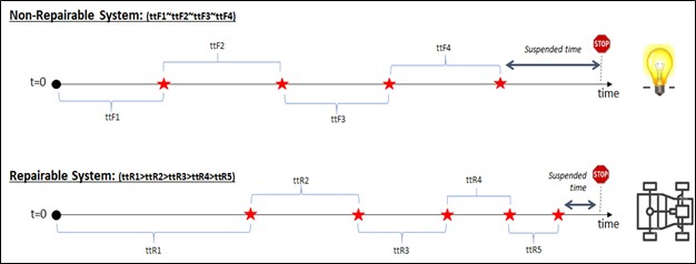
A repairable system is expected to fail one or multiple times over its life. It will be repaired and restored to as close as possible to its original functional state. However, it is very rare that it will be restored to an “as good as new” state because other parts of the system which have not failed yet are in a state of deterioration and will sooner or later fail. Subsequently, failures on this system will occur more and more frequently over time. A good example of a repairable system is an automobile.
On the flip side. A non repairable system is only used once. It is typically a consumable such as a light bulb or a bearing. Replacing the light bulb in its original location makes the lighting system in essence “as good as new”. And the new light bulb is expected to last as long as the last one. This is also called a “perfect” repair.
Hence, mathematically speaking, repairable and non repairable systems have to be treated differently when a study of their life cycle is conducted.
In summary, it is important for Reliability Practitioners to understand all the above-mentioned concepts as well as the pitfalls. So that they can assist the asset managers in making the optimal and best-informed decisions. The other challenge is to obtain a reasonable number of records in order to complete a robust reliability analysis of the system being considered. The Computer Maintenance Management System (CMMS) is typically the repository for those records.
Example of Restoration Factor Calculation
This example is obtained from the Reliasoft® Weibull++ Software library. Should the reader want to reproduce the calculations, the raw data is provided here. The calculations are performed using the Power Law. Repairable Systems follow the Power Law or Non-Homogeneous Poisson Process (NHPP). The life model results are provided in Table 1 below.
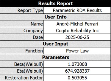
The Beta Parameter is slightly greater than one indicating increased degradation over time. In addition, and in line with the topic of this article, the Restoration Factor is at 50%. As mentioned earlier, the Restoration Factor indicates the degree to which the condition of a system will be restored after each repair. A value between 0 and 1 indicates the extent of the repair. In our case, the system will be “better than old but worse than new” after the repair. This is also called an “imperfect repair”.
In summary, the system considered here degrades over time. Failures will happen more and more frequently over time. Additionally, the repairs applied when a failure occurs, do not restore the system to its original state.
The questions the Asset Manager should consider are:
- Do we accept those finding as part of doing business?
- Is there a way to improve the effectiveness of the repairs. That is technician training, or improved maintenance procedures?
- Do we replace the equipment, re-engineer it or modify its operating environment?

Leave a Reply