
Broom” charts are reliability function estimates from different or successive production cohorts. Their differences may contain actionable information. How to quantify and use that information? This article provides an alternative to traditional Duane, AMSAA, and Crow reliability growth models, based on Cox’ proportional hazards model for test or field reliability data. This article provides:
- Broom charts that show reliability growth or deterioration
- Reliability growth references, including credit to my UC Berkeley professors
- Proportional hazards (PH) model(s) of reliability growth with vs. without lifetime data
- Suggestions for what to do about reliability deterioration
Suppose successive test samples or production cohorts have reliability growth or deterioration, caused by TAAF (Test, Analyze And Fix), configuration, environment, stress, or vendor changes, or ??? Suppose product cohorts have “proportional hazard” functions.
Biostatisticians estimate “hazard” functions, also known as failure rate functions in reliability lingo. Proportional hazard functions seem like a reasonable assumption, because generations of products have similar designs, parts, production processes, customers, environments, and lifetimes.
Reliability growth may not be MTBF growth, because most products’ lives are less than MTBF. We need ways to quantify reliability growth or deterioration, besides MTBF growth.
This article shows a PH model from Fred’s monthly production cohorts (ships)and their lifetime data in Kaplan-Meier Nevada table 1. It will also compare the PH model of Fred’s monthly failure counts, without lifetime data; i.e., cohort lifetimes vs. monthly return sums, using just monthly ships and failure counts, available from revenue and cost data required by GAAP, and some work.
Reliability Growth Illustrated?
Each line in figure 1 is a nonparametric reliability estimate from each months’ production (cohort). The figure’s legend is cohort production month (7 months of data). Later months’ lines are shorter because there is less data from more recent months. Shorter lines from more recent months’ cohorts appear to be more reliable. That’s because later cohorts’ (shorter lines) are higher than earlier cohorts
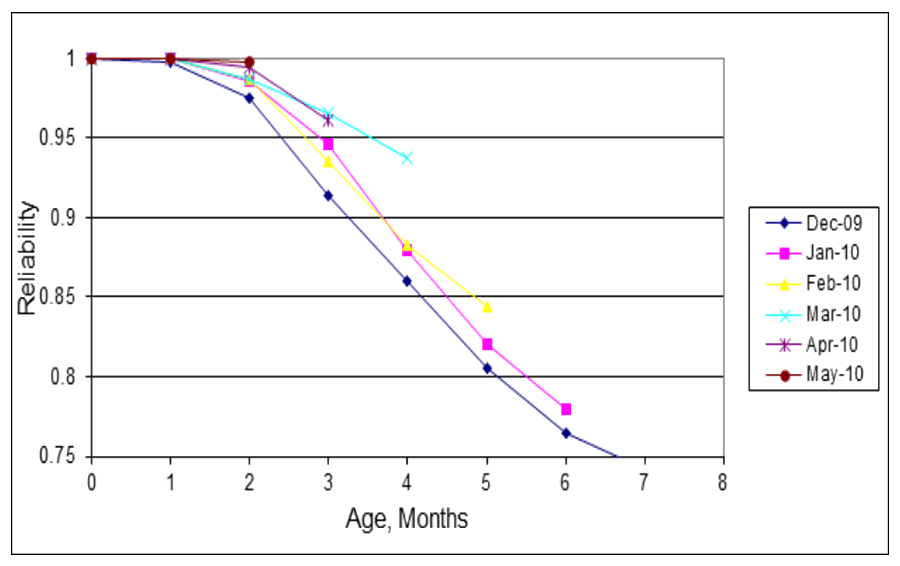
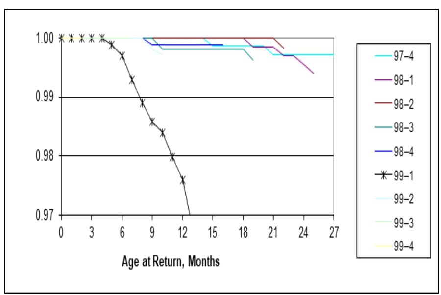
Figure 2 shows a broom chart of EEPROM reliability deterioration in January 1999. The EEPROM vendor shrunk the die size. Some January EEPROMs lost their little memories.
An alternative to broom charts for detecting problems is proposed by Wu and Meeker, “Early Detection of Reliability Problems Using Information from Warranty Databases”. They “…recommend a nonparametric approach based on warranty report counts modeled with a Poisson distribution with report intensities that depend on production period and number of periods in service. This is equivalent to fitting a piece-wise exponential distribution to the available data and does not require specification or use of a particular distributional form for the time-to-(failure)-report distribution.” This seems equivalent to the assumptions behind USAF Logistics Command actuarial methods and Poisson demand for engines circa 1974 [George 1978]. This does not quantify reliability growth in an actionable way.
Reliability Growth References
J. T. Duane observed that test time T divided by the number of failures N(T), T/N(T), plotted on log-log paper averaged linear. That meant MTBF=βT-α, where T is the total test time for parameters α and β. ReliaSoft says Duane published that in a 1962 paper [Duane 1964]. I found early reliability growth references by my UC Berkeley professors William Jewell and Richard Barlow. [Jewell 1963, Barlow and Scheur 1966].
It is convenient to have an MTBF growth model when testing to achieve an MTBF specification. That way one could predict a date on which reliability testing will show the MTBF specification will be met with specified confidence. Larry Crow extended the MTBF model to produce confidence limits on MTBFs. “The model analyzes the reliability growth progress within each test phase…” http://reliawiki.org/index.php/Crow-AMSAA_(NHPP)/. That inspired software, standards, and, more reliability growth articles. The reference by MacDiarmid and Morris contains a lot of reliability growth history and standards.
Duane-Crow-AMSAA reliability growth is really MTBF growth. It is for test-to-failure sample scenarios. It is irrelevant if reliability is good, because few field failures occur, at ages much less than MTBF. MTBF growth is irrelevant for infant mortality. MTBF growth in HALT (Highly Accelerated Life Testing) may not translate into reality, because highly accelerated testing may change the shape of failure rate functions.
Want to verify reliability (not just MTBF) growth resulting from test data, TAAF, or product or component improvements over time, tests, or renewal counts? See NIST/SEMATECH e-handbook “How can you model reliability Growth?” for some alternatives to MTBF growth, https://www.itl.nist.gov/div898/handbook/apr/section1/apr19.htm/.
Now there’s an R-program, “ReliaGrowR”, for Reliability Growth Analysis (RGA). The project implements core reliability growth models, including the Duane, Crow, AMSAA, piecewise NHPP (Non-Homogeneous Poisson Processes), and piecewise NHPP with changepoint detection! ReliaGrowR is available on the Comprehensive R Archive Network (CRAN) and was verified with example analyses, unit tests, and cross-platform checks to ensure reliability and stability [Govan]. ReliaGrowR models a piecewise linear NHPP model.
In a January 2026 memo, the USAF forbid the use of actuarial failure rate functions (equivalent to nonparametric reliability functions) and actuarial forecasts. The memo requires the use or average “Removals”/Time, (Failures/Time), https://accendoreliability.com/progress-in-usaf-engine-logistics/. Imagine reliability growth by monitoring average Failures/Time in successive calendar intervals. Good luck with that.
Reliability Estimates: Kaplan-Meier by Cohort
Table 1 shows Fred’s monthly sales or ships and corresponding monthly failures by cohort. The bottom row failure sums contain reliability information but do not indicate which cohorts they came from. Assume Fred’s monthly failures were dead-forever, not renewals or relevations. (“Relevations” are renewals or restorations to some good-as-old state [Krakowski].)
Table 1. Lifetime Data, in the form of Nevada Table, from “Nevada Charts to Gather Data”, by Fred Schenkelberg, https://accendoreliability.com/nevada-charts-gather-data/.
| Month | Ship | Jan | Feb | Mar | Apr | May | Jun |
| Jan | 3519 | 3 | 6 | 3 | 7 | 10 | 3 |
| Feb | 6292 | 4 | 8 | 20 | 35 | 24 | |
| Mar | 7132 | 8 | 14 | 25 | 31 | ||
| Apr | 5633 | 4 | 13 | 6 | |||
| May | 4222 | 5 | 8 | ||||
| Jun | 4476 | 6 | |||||
| Sums | 31274 | 3 | 10 | 19 | 45 | 88 | 78 |
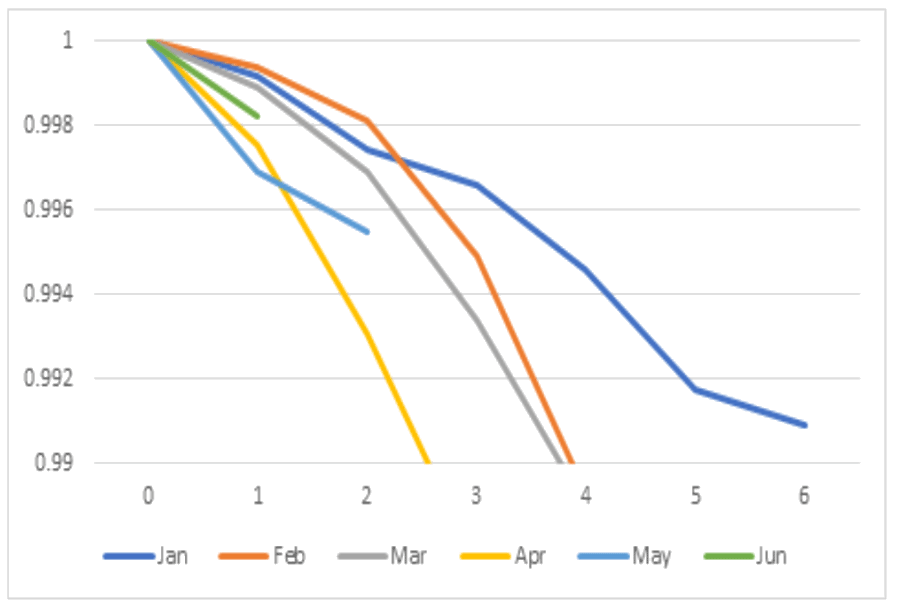
Reliability estimates in table 2 and figure 3, by cohort month of production, show deterioration and perhaps improvement in May and June! How to quantify cohort changes in reliability function estimates?
Table 2. Reliability estimates, by cohort, horizontally in each row, for ages 1-6 months.
| Month | Ships | 1 | 2 | 3 | 4 | 5 | 6 |
| Jan | 3519 | 0.9991 | 0.9974 | 0.9966 | 0.9946 | 0.9917 | 0.9909 |
| Feb | 6292 | 0.9994 | 0.9981 | 0.9949 | 0.9893 | 0.9855 | |
| Mar | 7132 | 0.9989 | 0.9969 | 0.9934 | 0.9890 | ||
| Apr | 5633 | 0.9975 | 0.9931 | 0.9875 | |||
| May | 4222 | 0.9969 | 0.9955 | ||||
| Jun | 4476 | 0.9982 |
Proportional Hazards Model of Cohort Reliability Growth
Cox’ proportional hazards (PH) models are popular in social sciences and medical science to assess associations between external variables (factors) and reliability, https://en.wikipedia.org/wiki/Proportional_hazards_model/. A PH model of failure rate function is a(t;z,β) = ao(t)Exp[z*β], where ao(t) is an underlying failure rate function, z could be 1, 2, 3,… cohorts, changes, improvements, fixes, etc., and β is a regression coefficient. Failure rate functions could remain proportional, because generations of products use similar designs, parts, production processes, customers, and environments.
Professor William Jewell proposed a failure rate function a(t; z) = β1*ao(t)+β2*a(t|z), where t is time between failures, and z is the time history of failures X(1), X(1)+X(2),…That is an example of a PH model, because ln[ao(t)Exp[z*β] = ln[ao(t)]+z*β, if ln[ao(t)] is linear.
Table 3. Check proportionality! The table shows cohort failure rates and their ratios of successive monthly cohorts’ failure rates (Jan/Feb, Feb/Mar, etc.) ratios, a(t; z)/a(t; z+1), z=1,2,…,5
| Age, Months | 2 | 3 | 4 | 5 | 6 | |
| Jan | 0.00085251 | 0.00031786 | 0.00217672 | 0.0024542 | 0.0017516 | 0.0013404 |
| Feb | 0.00047293 | 0.00085468 | 0.00091614 | 0.0015233 | 0.0010013 | |
| Mar | 0.00056439 | 0.00155595 | 0.00202924 | 0.0006999 | ||
| Apr | 0.00152489 | 0.00280722 | 0.00153532 | |||
| May | 0.00275587 | 0.00177040 | ||||
| Jun | 0.00162285 | |||||
| Ratios | Jan/Feb | Feb/Mar | Mare/Apr | Apr/May | May/Jun | |
| Age =1 | 1.34101 | 1.34159 | 0.26786 | 0.3564 | 0.73316 | |
| Age =2 | 0.56675 | 0.64709 | 0.90466 | 1.27589 | ||
| Age =3 | 0.45133 | 0.44109 | 0.63521 | |||
| Age =4 | 0.80717 | 3.11925 | ||||
| Age =5 | 1.72276 |
Ratios of actuarial failure rates vary! The average ratio of 0.974 is pretty close to 1.0, but the standard deviation is 0.729 and the coefficient of variation is 78%. Proceed with PH model fit anyway, for comparison without lifetime data in Nevada table 1, using just ships and the bottom row sums!
Use least squares to fit the cohort actuarial failure rates derived from table 2 reliability functions with the PH model (a(t;z,β)=ao(t)Exp[z*β]), by changing β. Minimize the sum of squared errors (SSE) between estimated cohort actuarial rates and PH model. The minimal β=0.11177 indicates failure rate increases with cohorts, confirming the reliability decrease in figure 3!
Table 4. Least squares to fit the PH model to the cohort actuarial rates from table 3: a(t; z,β)=ao(t)Exp(z*β) where ao(t) is the actuarial failure rate from the Kaplan-Meier reliability estimates from table 2 and z=cohorts 1,2,…,6.
| 1 | 2 | 3 | 4 | 5 | 6 |
| 0.001037 | 0.00116 | 0.001297 | 0.00145 | 0.001622 | 0.001813 |
| 0.002005 | 0.002242 | 0.002507 | 0.002803 | 0.003135 | |
| 0.002257 | 0.002524 | 0.002823 | 0.003157 | ||
| 0.004861 | 0.005435 | 0.006078 | |||
| 0.003920 | 0.004384 | ||||
| 0.000961 | |||||
| 3.5704E-05 | <- SSE | 0.11177 | <- β |
Without Lifetime Data?
Lifetime data is not required to quantify reliability growth, despite what people think! LinkedIn poll results: 91% said lifetime data is required to estimate reliability or survival functions, and 9% said lifetime data is NOT required. Nobody said “Don’t Know” [George, May 2023].
Periodic ships and returns or failure counts (bottom row sums from Nevada table 1) are statistically sufficient to make nonparametric reliability estimates [George, May 2022]. The ships and returns data could come from revenue and service cost (e.g., spares sales), data required by GAAP.
To fit the PH model, compute reliability and failure rate function estimates from successive cohorts, excluding earlier cohorts and their failure sums as shown in table 5. Figure 4 plots the maximum likelihood reliability function estimates. These estimates should not be compared with figure 3 reliability estimates, because cohorts are defined differently. Nevertheless, figure 4 shows reliability deterioration similar to figure 3.
Table 5. Ships and column failure sums starting with cohort 1 rows 2-7, cohort 2 rows 8-12, etc. from Nevada table 1. The “Failures” column rows 2-7 are same as table 1 bottom row sums.
| Month | Ships | Failures |
| Jan | 3519 | 3 |
| Feb | 6292 | 10 |
| Mar | 7132 | 19 |
| Apr | 5633 | 45 |
| May | 4222 | 88 |
| Jun | 4476 | 78 |
| Feb | 6292 | 4 |
| Mar | 7132 | 16 |
| Apr | 5633 | 38 |
| May | 4222 | 78 |
| Jun | 4476 | 75 |
| Mar | 7132 | 8 |
| Etc. | 5633 | 18 |
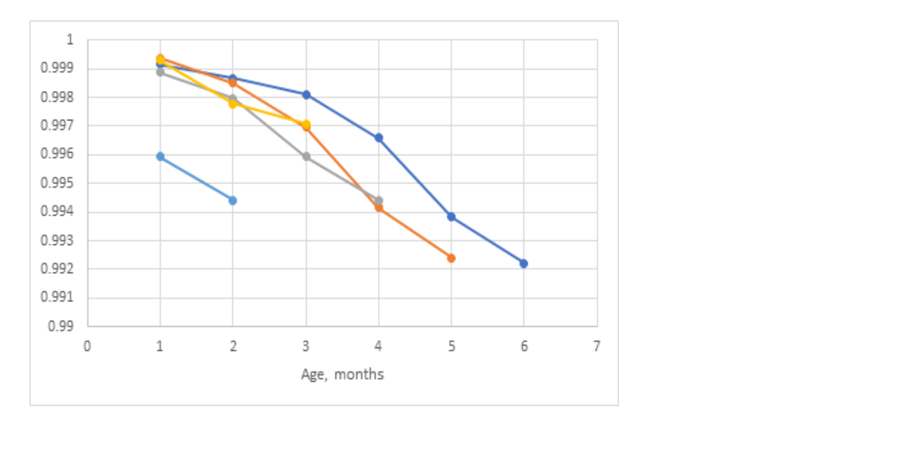
Figure 4. Reliability function estimate computed from successively later cohorts. Longest line is from Jan-June and shortest line is from June.
Table 6. Ratios of successive failure rate function estimates, without lifetime data.
| 1/2 | 2/3 | 3/4 | 4/5 | 5/6 |
| 1.80262 | 0.37191 | 2.37597 | 1.61104 | 1.74926 |
| 0.83795 | 0.54930 | 0.45147 | 2.17652 | |
| 0.37012 | 0.55427 | 1.32170 | ||
| 0.55333 | 1.58564 | |||
| 1.69817 |
Table 7. Computes PH β Using Solver to minimize SSE between cohort failure rate function ratios (similar to table 3) and proportional hazards model ratios (shown).
| 1 | 2 | 3 | 4 | 5 |
| 0.001008 | 0.001190 | 0.001407 | 0.001663 | 0.001966 |
| 0.000559 | 0.000661 | 0.000781 | 0.000923 | |
| 0.000667 | 0.000789 | 0.000932 | ||
| 0.001802 | 0.002130 | |||
| 0.003257 | ||||
| 8.564E-06 | <- SSE | 0.167108539 | <- β |
Ratios of actuarial failure rates vary! Average ratio 1.2006 is pretty close to 1.0, but the β with lifetime data by cohort = 0.11177 vs. β without…= 0.16711. Note also SSE=8.564E-06 without lifetime data is smaller too: SSE=3.57E-05 with lifetime data in Nevada table.
There’s a price for not having lifetime data. β-without lifetime data = 0.16711 may exaggerate increases in failure rate function estimates. Maybe that’s good for early warning. Maybe it’s biased by earlier, larger cohorts. At least it quantifies trend in failure rate function estimates.
If you don’t have lifetime data, ships and returns counts are statistically sufficient and available from revenue and service cost data required by GAAP (and some work)! Is the difference in β with vs. without lifetime data worth the cost of lifetime data? Lifetime data requires tracking products and service parts by name, serial number, and ages at first use to first failure and survivors’ ages. Lifetime data presumes dead-forever, and may not include renewal or recurrent processes.
Try the PH model [Evanco], for comparison without lifetime data, for software. For other attempts, see articles by Folorunso et al. and Strunz et al. PH models for factors have FDA approval!
What could We Do About Reliability Deterioration?
If reliability is deteriorating: Why? What did it? When? How to fix it? Cost? Broom charts may identify outlying cohorts as in figure 2. Use “Statistical Reliability Control” [George, Aug. 2023].
You could relate β to bang per buck, dβ/d$$$, for alternative improvements and their $$$ costs per unit change in β, and use budget constrained optimization to maximize reliability as a function of β. β is simple, scalar; one measure for all cohorts, although later cohorts are smaller and have shorter lifetimes and fewer failures. You could make PH parameters z and β into vectors and a(t; z, β(j))=ao(t)Exp[Σβ(j)*z], j=1,2,… to incorporate more z-factors besides cohort in the PH model.
Kullback-Leibler divergences (bits), as in “Statistical Reliability Control”, might be a better indicator of reliability deterioration than a proportional hazards model, https://en.wikipedia.org/wiki/Kullback%E2%80%93Leibler_divergence/. Kullback-Leibler divergence is a pairwise multiple measure of differences between old probability density functions p(t) and new q(t), Σp(t)log(p(t)/q(t)), for some range t=1,2,…k. Kullback-Leibler divergence is intended for pairwise comparisons of sums of probability density functions, Σp(t) and Σq(t), over same range(s), usually Σp(t) and Σq(t) =1.0. In the reliability growth context, you may only have new q(t) for small t = k, maybe t = cohorts k-1,k.
What Can You Do to Improve Reliability?
Ask yourself and customers if the product’s reliability is good enough? That requires knowing the product’s reliability: https://accendoreliability.com/reliability-from-current-status-data/. I have had some success by offering to share a vendor’s part’s reliability estimate, in our products, if they would share all their customers’ ships and returns (failure) counts. I provided estimates of vendor’s part’s reliability, in our products vs. vendor’s part’s population reliability.
Designers claim that their designs determine reliability. A Sun Computer design engineer asked, “Why do we need you? We design reliability into our products.” I gave him nonparametric estimates of field failure rate functions for several products (1996), showing infant mortality and wearout beginning within 12 months. Process, shipping, installation, training, and usage all conspire to deteriorate design reliability.
What if Renewal Process?
Duane-Crow-AMSAA reliability growth is NOT for renewal, recurrent, repair, or replacement process data. Reliability growth implies renewals are better than old. What if recurrent processes have independent but not identical distributions for successive lifetimes? Assume Cox’ proportional hazards model of failure rate functions for successive lifetimes? It’s been done before.
MCF, is the Mean Cumulative (failures) Function, E[N(t)], the expected value of the number of failures in a calendar or operating time t. MCF is for systems that are repairable or recurrent processes [Nelson, Ascher and Feingold, Trindade]. Reliability growth or deterioration is shown by curvature of the MCF as time progresses. But what if you don’t have lifetime data?
What if successive failures are renewal (independent, good-as-new, lifetimes) or relevation processes? Relevation means repair after failure brings product back to life good-as-old or somewhere between good-as-old and good-as-new or perhaps even better. Refer to “Hysterecal Renewal Processes” for some examples [George, Aug. 2023].
Stay tuned to www.accendoreliability.com for how to estimate cohort proportional hazards reliability growth for renewal or recurrent processes, with or without lifetime data!
Reliability Growth References
Barlow, Richard E. and Ernest M. Scheuer, “Reliability Growth During a Development Testing Program,” Technometrics, Vol. 8, pp. 53-60, 1966
Larry H. Crow, “Confidence Interval Procedures for Reliability Growth Analysis”, Technical Report No. 197, June 1977
J. T. Duane, “Learning Curve Approach to Reliability Monitoring”, IEEE Transactions on Aerospace, vol. 2, pp. 563-566, 1964
Robert Easterling, “The Assessment of System and Component Reliabilities Based on Both System and Component Test Results”, Note 3 of Sandia Lab Probability and Statistics Notes, Dec. 1970
Easterling, R. G., and R. R. Prairie. “Combining Component and System Information.” Technometrics, vol. 13, no. 2, pp. 271–80. JSTOR, https://doi.org/10.2307/1266789/, 1971
Robert G. Easterling, Mainak Mazumdar, Floyd Spencer, and Kathleen Diegert, “System-Based Component Test Plans and Operating Characteristics: Binomial Data”, Technometrics, (33) 3, March 2012
P. B. Govan, “ReliaGrowR: Modeling and Plotting Functions for Reliability Growth Analysis,” Reliability and Maintainability Symposium (RAMS), Miramar Beach, FL, USA, pp. 1-6, doi: 10.1109/RAMS50514.2026.11424445, 2026
Joe Alex Granado and Tongdan Jin, “Spare Provisioning for System Maintenance under Reliability Growth-A Case Study”, INFORMS meeting, Austin, TX, Nov. 2010
William S. Jewell, “A General Framework for Learning Curve Reliability Growth Models,” UC Berkeley Operations Research Center, AFOSR-81-8122, April 1963
William S. Jewell, “Reliability Growth as an Artifact of Renewal Testing”, University of California, ORC 78-9, Operations Research Center, Berkeley, June 1978 or October 1978
Krakowski, M. “The Relevation Transform and a Generalization of the Gamma Distribution Function”, Revue Francaise d’Automatique, Informatique et Recherche Operationnelle, vol. 7 , pp. 107–20, doi:10.1051/ro/197307V201071, 1973
Preston R. MacDiarmid and Seymour F. Morris, “Reliability Growth Testing Effectiveness”, RADC-TR-84-20, AD-A141 232, Jan. 1984
MIL-HDBK-189c, “Reliability Growth Management”, June 2011
MIL-STD-1635, “Reliability Growth Testing”, Feb. 1978
ReliaSoft, “Reliability Growth & Repairable System Data Analysis Reference”, https://help.reliasoft.com/reference/reliability_growth_and_repairable_system_analysis/pdfs/rga_ref.pdf/, 1992-2005
Huaiqing Wu and William Q. Meeker, “Early Detection of Reliability Problems Using Information From Warranty Databases”, March 2001
MCF References
Stephen A. Smith and Shmuel Oren, “Reliability Growth of Repairable Systems”, Naval Research Logistics Quarterly,Vol. 27, Issue 4, pp. 539-547, Dec. 1980
Jan Block, Alreza Ahmadi, Tommy Tyrberg, and Uday Kumar, “Fleet-Level Reliability Analysis of Repairable Units: A Non-Parametric Approach using the Mean Cumulative Function”, International Journal of Performability Engineering,Vol. 9, No. 3, pp. 333-344, May 2013
David Trindade and S. Nathan, ”Field Data Analysis for Repairable Systems: Status and Industry Trends”, In: Misra, K.B. (eds) Handbook of Performability Engineering. Springer, London. https://doi.org/10.1007/978-1-84800-131-2_26, 2008
Harold Ascher and Harry Feingold, Repairable Systems Reliability: Modeling, Inference, Misconceptions and Their Causes, Marcel Dekker, 1984
References to PH and Alternatives?
David R. Cox, “Regression Models and Life-Tables”. Journal of the Royal Statistical Society, Series B. vol. 34 (2), pp. 187–220, doi:10.1111/j.2517-6161.1972.tb00899.x, JSTOR 2985181, MR 0341758, 1972
W. M. Evanco, “Using a Proportional Hazards Model to Analyze Software Reliability,” STEP ’99. Proceedings Ninth International Workshop Software Technology and Engineering Practice, Pittsburgh, PA, USA, pp. 134-141, doi: 10.1109/STEP.1999.798487, 1999
Serifat Folorunso, Richard Oluwaseun Kehinde, Ibrahim Arionola Fayemi, and Sukurat Salam, “Deep Learning-Based Survival Analysis and Recurrence Prediction in Breast Cancer Patients Using Clinical and Genomic Data,” SCOPUA Journal of Applied Statistical Research, Vol.2, Issue 1, https://doi.org/10.64060/JASR.v2i1.4, March 2026
Richard Strunz and Jeffrey W. Herrmann, “Planning, Tracking, and Projecting Reliability Growth A Bayesian Approach”, Proc. Ann. Reliability & Maintainability Symposium, 2012
References by L. L. George
“Revaluation of the Air Force Actuarial Method for Forecasting Engine Requirements,” Proceedings of the Annual Reliability and Maintainability Symposium, pp. 7-10, January, 1978
“Credible Reliability Test Planning”, https://accendoreliability.com/credible-reliability-test-planning/, March 2022
“How Can You Estimate Reliability Without Life Data?”, (Myron Tribus) https://accendoreliability.com/can-estimate-reliability-without-life-data/, May 2022
“Is Lifetime Data Required”, https://accendoreliability.com/poll-is-life-data-required/, May 2023
“Statistical Reliability Control”, https://accendoreliability.com/statistical-reliability-control/, August 2023“Proportional Hazards Reliability of Hysterecal Recurrent Processes”, https://accendoreliability.com/proportional-hazards-reliability-of-hysterecal-recurrent-processes/, August 2023

Leave a Reply